Rate and Master Equations
Table of Contents
Introduction
This is part 1/? of a series of posts on the theory of “reaction networks”, a.k.a. “Petri Nets”, a.k.a. “mass-action kinematics”. For the most part this material will be assembled from various links on John Baez’ page. Almost nothing here is my own work, but I will be restating it in my own words and partially in my own notation.
My own interests are in:
- Elementary examples of parts of quantum-mechanics and statistical-mechanics, e.g. Fock Space, and in decomposing these theories into simpler ones.
- The relationships between descriptions of the same system at levels of abstraction, with a renormalization flavor.
- The zoo of equilibrium behaviors of dynamical systems, and how they relate to the underlying parameters
- Generating function methods, wherever they appear.
- The opportunity to develop methods of diagramming high-dimensional spaces.
Reaction Networks
A “reaction network” is a graph whose edges represents “reactions” (or “processes” or “transitions”) between different “complexes” (or “combinations” or “tuples”) of “species” (or “molecules” or “compounds”)
Here’s a generic example:
The network represents a set of “processes” by which a system can evolve. From it we can produce various mathematical models, e.g. a set of coupled differential equations for “concentration” of each species, where we assert that each process
As no other reactions occur, any state which is not accessible via some sequence of the reactions in the network is unreachable. The set of possible states is further constrained by the rate constants, meaning that some states may turn out to be attractors while others are dynamically unreachable.
Here’s an example of a chemical network:
This system’s behavior is oscillating. You can sort of see this just by inspecting the formulas: the first reaction is a positive feedback loop fueled by
Here’s a Lotke-Volterra predator-prey model:
where
The system of equations is:
And here is a simple model of disease spread:
where
In this (very simple) model, “infections” can be observed either to die out rapidly (the number of sick goes quickly to zero) or will grow into an epidemic, where the rate of new infections equilibrates with the rate of deaths. Which phenomenon occurs depends on the values of the rate constants
Evidently reaction networks imply a large class of “model systems” which exhibit various system dynamics, among them, the cycles and bifurcations seen in these examples.
Levels of Abstraction
I want to emphasize here at the outset that a “reaction network” describes a set of processes, which can then be “translated” into equations in various ways—in particular, at different “resolutions”, “levels of analysis”, or “levels of abstraction”.
-
Equilibrium. The highest level of abstraction. Here we characterize a system by its equilibrium or long-time behavior, which might be an attractor state, but also might include more complicated behaviors like cycles.
Examples: Equilibrium concentration of a chemicals in solution. Thermodynamics as equilibrium stat-mech.
-
Mean Dynamics. This is the entrypoint for most analysis of a reaction network: we translate the network into a differential equation related the total populations or concentrations. This is called “Rate Equation”, which is an ODE in species counts
. We can then analyze this ODE to determine its asymptotic behaviors, stability, bifurcations, etc., which can tell us things at level 0. Examples: The Lotke-Volterra and epidemic examples above. Quantum mechanics in the semiclassical limit.
-
Stochastic Dynamics. At this much-lower level of abstraction, we can translate the network into the time-evolution law for probability distributions over states with specific “occupation numbers” for each species. This is a far-more granular description than the mean-dynamic level, and there could be intermediate levels. Generally this description of the system is far less tractable, but in some ways it is more amenable to analysis, and as we’ll see can be related to the Rate Equation at level 1.
Examples: the Shrodinger equation.
-
Histories, Timelines, or Sequences of Reactions. At a lower-level still would be a characterization of the state as a particular sequence of reactions, with which we can associate some probability-weight or “amplitude”. The weighted sum of all possible timelines we expect to leads to the higher-level characterizations of the system. But this level of analysis is particularly suited to questions like: what is the probability for a transition between specific starting and ending states?
Examples: a diagram in a path integral, in QFT. I also think of “programs”, in the sense of a sequence of expressions in an abstract language. Specific sequence of mutations in genetics.
-
Micro-scale Dynamics. At the lowest level of analysis we have the interactions of individual particles. At this level the reaction network doesn’t tell us anything; in fact this is the level where you might calculate the rate constants used at higher levels of analysis by computing scattering cross sections from the underlying dynamics. Or perhaps we can use statistical-mechanics methods to find a density-of-states or partition function.
Examples: Hamiltonian mechanics of interacting particles in a gas. Individual vertexes in QFT.
Most of the theory here will concentrate on the three highest levels of analysis. I spell all of this out because, first, I think it will be a good way to organize these ideas, but in particular because, for me, the most interesting thing about reaction networks is as a model system for understanding the relationships between the different levels of abstraction.
With this we will begin at “Level 1”: the mean dynamics, as expressed by the Rate Equation.
Level 1: The Rate Equation
Anatomy of a Rate Equation
A reaction network is most simply seen as encoding a differential equation called the Rate Equation of the network.
Here is the example from above again:
We translate into the following set of coupled diff-eqs:
When we want to iterate over reactions, we’ll index by
In the differential equation, the variables
Concentrations are always non-negative real numbers—we think of the rate equation variables as representing the time-dependence of averages or expectations rather than integer numbers of molecules or organisms.
The rate of a reaction depends on the product of the concentrations of its inputs only, e.g. our first reaction
The coefficients like
The specific combinations of species appearing on either side of each reaction are the complexes of the network. These are, conceptually, the “clusters” which have to come together for the reaction to occur.
We will index complexes by a lower-case
, so , , and the full tuple is . , so and the full tuple is .
The difference
We could try to write the Rate Equation as a matrix equation:
…but this won’t be very useful because the matrix isn’t square—instead it has dimension
The general formula for a rate equation is a sum over reactions, where
We will sometimes use the symbol
Example: Solving a Rate Equation
For any particular network you could attack the corresponding Rate Equation with the methods of standard differential equations. In general we can’t hope to find exact solutions; the goal of such analysis is usually to make “level 0” statements characterizing equilibria and long-time behavior. But it will be helpful to see the general shape such an analysis takes with a worked example.
As a demonstration of what it takes to analyze a particular Rate Equation, I’ll look at the epidemic model from above, where, again
This leads to the following system of equations:
The deltas are
We can also write this as a matrix equation where the input is a vector of complexes and whose output is a vector species of:
To solve this, it helps to note that both processes conserve the total population. Hence we can define a conserved quantity
Now to solve it. This system is simple enough that it admits an exact solution by way of the following trick. We observe that the
Then the solutions for
And we can make use of the fact that
We now define parameters to make this dimensionless. If we define
And now we define constants
We arrive at a fairly simple first-order differential equation, which is most easily analyzed by observing that
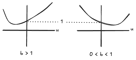
Then the full system
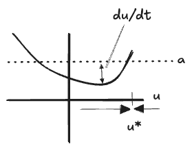
Apparently:
- When
, meaning , is a fixed point: a healthy population can’t suddenly get sick. - When
or , the model develops an “attractor” fixed point —an eventual “death toll”—and while the value of the attractor increases slowly as a function of the initial condition (through , which isn’t really independent of ), it increases very quickly as a function of the “rate of transmission” relative to the rate at which sick patients die off ; represented by .
From here you could go on to calculate the location of the fixed point as a function of the parameters and the initial conditions, or the timescale of convergence to the fixed point, or you could modify this comically-simple model to include behaviors like “getting better” and “quarantining”. But it is adequate to demonstrate the typical behavior of reaction networks: fixed points appear and move around the parameter space as a function of the rate constants.
Tuple Notation
All the species indices in the rate equation are not particualrly easy to read. Some of the literature chooses to clean this up by omitting the species index entirely, asking us to remember which terms refer to species (which obey special rules) and which do not. I want to take a different approach and represent indexing-over-species as an overbar
A tuple over species
Tuples can be added or subtracted, and it will occasionally be useful to take a dot-product:
We’ll also define operations on tuples which do not have vector analogs. Most operations which would not be defined on vectors we implement by applying component-wise, then multiplying all of the components of the result:
Note that the last line is a succinct way to write a multinomial coefficient
We will need a couple more non-standard operations as well.
First we have the “falling power”, which works for integers or tuples:
The last line indicates that the falling power could be related to a multinomial coefficient with both arguments tupled, but this seems a little too wacky, so we won’t use it.
Note that
Next we have the scalar product of more-than-2 tuples, which we write as a chain of dot-products:
And lastly we implement inequality between tuples, which can be seen as a shorthand for “logical AND” or as a product of indicator functions. We won’t attempt to find a notation for “OR”.
With all of this notation, and
The Rate Equation on column vectors looks like this:
We want to write this as a “tuple equation”, just as we do for vectors, representing a system with one equation for each tuple index
We immediately encounter a weakness of the notation, unfortunately—we would like to write this term as
An alternative to all of this would be to use an Einstein-like notation, with the rule that tuple components multiply for any tuple index appearing on only one side of the
I’m going to stick with tuples, though—we’ll get a lot of use out of them.
Our concise Rate Equation is therefore:
But in fact the tuple notation will not be all that useful for rate equations—it will serve us better at the next level of abstraction.
Level 2: The Master Equation
Stochastic Dynamics
In one sense the Rate Equation is a direct translation of the information in a reaction network. But in most cases this should be thought of as an approximation of the underlying physical system, in a few ways:
- The rate constants
are either estimated from measurements, or, if they’re determined from the underlying physics, are probably approximations which only capture the highest-order interactions - The law that reactions occur with rate
is itself only approximately true - The initial conditions are only approximate measurements and therefore represent a peaked distribution of species numbers
, which is in actuality discrete rather than continuous, and may be quantum-mechanical
We could imagine trying to “undo” the abstraction along any of these axes. Here we’ll take the first two as givens—as assumptions of the “reaction network” class of models, essentially—and only broaden our view along the third axis.
Instead of concentrations, we’ll now consider the time-evolution of a probability distribution over the exact particle numbers.
A “state” will now be a distribution
This is a “stochastic” dynamical system, but will turn out to closely resemble a quantum-mechanical wave function, with the Master Equation corresponding to the Shrodinger Equation. 1
Following that analogy, we can represent a full state by an expression which looks like a wave function:
Note that in the stochastic case, the coefficients
Our “Master Equation” will represent the time evolution of this distribution by a Hamiltonian-like operator:
The solution can be found for a given initial condition as a time-evolution operator which is just the matrix exponential of the generator
Now we’ll build it. First we need to represent our reactions in the occupation-number basis. We’ll use off the same example from the beginning of this essay:
Each reaction
How do we represent the rate of a reaction? Reaction
- The prior probability, of
which is - The rate constant
2 - The number of ways to choose all of the reaction’s inputs
out of all the candidates in state , which is the tuple “falling power” introduced above:
We also have a condition that
Then the total rate of reaction
Our time-evolution generator will consist of one of such term for each initial state
This form implies that our generator matrix
The full Master Equation is:
We can isolate the generator of time-evolution
The Master Equation on Generating Functions
Now, rather than representing our state by a sum over occupation-number basis elements
You could motivate this in a few ways:
- Out of a general love for generating functions (like my own)
- Or, by analogy to the Rate Equation
, which involved powers of a species tuple as well, perhaps hoping to derive the Rate from the Master (we’ll try this in a bit) - Or, by observing that falling powers
, which we used above to count the “number of ways of choosing in the reaction inputs ”, corresponds exactly to the coefficients you get when taking derivatives of the monomial3:
Guided by this observation, we’ll take our quantum-mechanical analogy even further by defining a “creation” operator
The implementation of
We’ll write each of these as a tuple over all species
We can also define a number operator
The
Applying multiple
So we can also define the “falling power of the number operator
… and that is everything we need to represent the Master Equation as a time-evolution operator in the generating function representation:
This is a sum across reactions
Read this as:
- First, consume the inputs
from the input state ”, which gives the state times the original probability and a coefficient representing the probability of this reaction occuring. - Then, in parallel:
- move to the new state
and add all the probability - subtract all of the probability from the original state
- move to the new state
For comparison, here is the original original Master Equation, with
I prefer the operator version. There’s one fewer
Finally, in either representation, we can implement time-evolution by exponentiating this thing and acting on an arbitrary state:
Time Evolution as a Path Integral
Now we’ll briefly dip our toes into the next level down the ladder of abstraction.
One advantage of the operator formulation is that it lends itself to a path-integral-like interpretation, as follows. Observe that
Carrying out the powers leads to terms with sequences of
- the number of ways to choose candidates for those sequences: a product of terms
. - the probability that those reactions occur independently, which gives a product of factors
for each reaction , representing the underlying hypothesis that all reaction occur at independent rates over time. - a correction
for each sequence of reactions, which (I think) avoids an overcounting which arises because permuting the sequence of reactions is equivalent to permuting the times at which those reactions occur
For example, if our network looks like this:
Then we have two “processess”
For this sequence the combinatorial term
We can draw diagrams for three of these combinations; the other 3 choose the same two inputs into
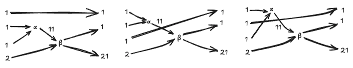
Observe that in each case one of the “1” particles passes through untouched, being affected by only the identity term of
These are something like Feynman diagrams. They’re mostly a conceptual aid at this level, but they could be useful when analyzing small-
Once again the most interesting result might be the light this can shed on quantum-mechanics through the analogy. It has always felt to me that QM was a tangled mess of concepts which, individually, are not all that complicated. Once you have an elementary example of each, the full theory ought to “factor”, with the particulars of quantum physics entering at clearly-delineated points. This could at least be an aid to pedagogy; of course any improvement to pedagogy can also improve the reach of pedagogy. If we dare hope for more, we might aim to better “compress” the body of physics knowledge better in the minds even of experts, letting all see further and more-easily grasp subtleties than in the current presentation. If!
-
In quantum mechanics one might arrive at the same thing by first considering some
underlying single-particle wave functions; then restricting to only anti-symmetric or symmetric combinations (a Fock Space), and then switching to the occupation basis. We won’t run into those symmetrization questions because we are not trying to say anything about spatial wave functions. (I imagine quantum mechanics would come out cleaner by starting with the occupation numbers. Spatial wave functions are the complicated part. These occupation-number equations will not be difficult to write down, as we’ll see.) ↩ -
Here we are effectively modeling the dynamics of this stochastic system as though particles encounter each other at some fixed global rate, probably proportional to the overall density, with 2-particle interactions occurring
, 3-interactions , etc. The rates of individual reactions then depend on which combinations of particles participate in the interaction. Obviously a realistic chemical model would have some global “temperature” parameter determining the rate at which interactions occur globally, but we will ignore that in the interest of generality; effectively we are rolling it into the definitions of the rate constants . If you want to split out, you could add a fourth factor to this list . ↩ -
Apparently, the coefficient in a derivative
was always counting the number of ways to choose which copy of to remove—a fact which I may have learned in calculus class, but have long since forgotten. ↩ -
Note the quantum-mechanical analogy. For
, the uncertainty principle is just this same identity . It almost looks like the in in Q.M. doesn’t need to be there—it has the effect of making operate correctly on functions of the form , where it gives . To me, this looks like yet another feature of Q.M. which could be “factored out” of the theory—I need to be keeping a list. ↩
Comments
(via Bluesky)