The Action—as in “The Principle of Least Action”—has been washing around in my mind only partially digested ever since undergraduate physics. This thing:
It’s not that it doesn’t make sense. I’ve seen the arguments, I know how to use it, it works well. The problem is harder to put a finger on; it’s something like: the “mode of argument” or “standard for proof” of a physics education switches partway through mechanics class. Until then the mode relied on physical intuition first, never stepping far out of sight of the physically-interpretable, and having as its ideal a derivation of physical law from reality, rather than a fitting of mathematics to reality. Then one encounters the Lagrangian , and the Euler-Lagrange equations , which is justified on the grounds that it works well—but what is it? What is , physically? Then we zoom out again to introduce , and justify the E-L equations from —again not by a derivation but by simply saying “do this, it works”, and without restoring contact with physical intuition. By then you’ve lost me. That’s two sketchy steps on top of each other, which is one too many for me. I thought I’d get over it, but I never did.
Here, then, are the missing arguments from mechanics class.
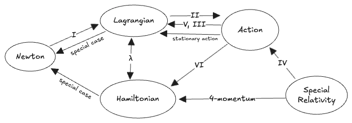
Here’s a map of where we’re headed:
The Roman numerals are section numbers; the other labels refer to the textbook derivations. The sections largely stand on their own, but are given in a logical order.
I. From Newton to Euler-Lagrange
My first complaint about the derivation of classical mechanics is that we receive the Lagrangian and the Euler-Lagrange equations from “on high” and then proceed to show that these reproduce Newton’s laws. Surely we should be able to go the other way, at least heuristically.
The following argument is from a 1972 paper “Geometric Nature of Lagrange’s Equations” by Beers, but also appears in some graduate texts like Goldstein. I want to record it argument for completeness, but the reader may want to skip to section 2.
We start with some mass and a motion described by , obeying Newton’s laws, in particular N2 . In short, with elementary physics.
Then we ask: what does this same motion look like in any other coordinate system ? This could be motivated in various way: maybe these are spherical coordinates, or they could be chosen to factor a problem into uncoupled subproblems, like the radial and angular components of planetary motion. Or for some particular problem, the could be defined so that motion along one or more of the is prohibited by a constraint—the radial direction for a bead constrained to a hoop, in that example. Why we want to re-parameterize doesn’t matter for the argument.
We write the original coordinates as a function of the new ones , whose derivative is:
That is, relates to in the same way that relates to , by a factor of which is just the Jacobian of the coordinate transformation.
We’ll now express N2 in the reference frame of the by projecting both sides onto columns of the Jacobian . This is:
Note the l.h.s. is not an expression for ; instead we are projecting onto the local frame induced by variation of the coordinates. This is admittedly a rather arbitrary thing to do at this point.
It will be easier to follow the rest of the argument if we work on just one of the components , which relate to only one of the new coordinates :
This expression has two factors of in each term, which suggests that this expression can be arranged to give a term like . Proceeding:
Our clever choice of has led directly to the kinetic part of the Euler-Lagrange equations in the new variable. The rest of E-L we can find in the forces. We project the generic forces into the same direction to give the “generalized forces” :
If any of the forces can be written as gradients of potentials, then projecting is simply a change of coordinates:
Let us also treat, for generality, a constraint on motion of the form . We separate out the corresponding constraint force from our list of forces. The constraint force is only ever in the direction of the gradient of the constraint, and takes a value proportional to some unspecified function equaling whatever it needs to to enforce the constraint. (The units of depend on the units of the constraint). Then a projection of this onto becomes a coordinate transformation of the gradient in the same way as :
Note the term acts like the gradient of a “constraint potential” , but the other term produced by the product rule for derivatives vanishes because the constraint in all actual states of the system.
The constraint force is therefore just another force—it could just as easily be represented by a —but we’ll continue to keep it separate for clarity.
In all we get:
And there we have the Euler-Lagrange equations of . No virtual forces, no virtual work, no “just introduce and show that it works”—one fairly straightforward calculus manipulation bridges the gap. The only trick part is guessing where to start—the expression was necessary to produce the term .
I’ve included a generalized force and a constraint force for completeness, but you don’t need those to get . The only really sketchy step was early on when we wrote . I’m not sure how to make the case for this, but it appears to be a standard.
We also get for free, without having to assert it arbitrarily.
In any case, that is the first “missing derivation”: and the E-L equations, directly from Newton.
II. From Euler-Lagrange to
Now we will start by taking the Euler-Lagrange equations for granted as representative of Newton’s laws in any frame. My next goal is to derive the form of itself and to come up with something representing the stationary action principle, without having to assert it out of the blue.
Consider a physical path beginning at a fixed point in , and ending at a fixed time but an unspecified endpoint . We assume it is a physical trajectory obeying the Euler-Lagrange equations everywhere; then we imagine varying the initial velocity ) and observing how the endpoint of the path varies.
We start with the E-L equation
and multiply by , representing the variation in the trajectory as the endpoint is varied. I think of “pulling” the endpoint, which should have a locally-smooth effect on the path and on its initial velocity.
Proceeding:
On the third line we used , which is standard but non-obvious to me. On the third-to-last line we used the fact that we had defined specifically as the variation in while fixing . Our final result is the equality of two things, as of yet uninterpreted: at the endpoint of the path, which we knowingly name , and over the whole path, which we knowingly call .
In other words: whatever this integral means, its differential with respect to the endpoint of some path, known to otherwise obey the E-L equations, depends only on the value of at the endpoint. Its full differential with respect to the endpoint then must have the form:
Now we’ll look for the other partial derivative. We imagine now fixing the endpoint and varying the end time . Then:
We have knowingly given the name for energy. (I will use rather than for Hamiltonian, unless considering as an explicit function of .) We used the previous result and also assume that the final velocity of the path is unaffected by the variation in the endpoint (which is a little suspicious).
In all, our differential with respect to the two coordinates of the endpoints of a physical path is:
Note this is equal to , and if we rearrange:
we find that the term is just the source of the minus sign in .
If we now went through the same derivation for a variation of the initial point of the path we would get the opposite signs. The full differential of with respect to its endpoints is therefore:
We can get from here to an explicit “stationary action principle” as follows: if we consider some larger interval , we ask what the variation of would be w.r.t. an intermediate point , given that the path in both halves of the interval separately obey E-L equations. The first half would then give , while the second half would give , for a total variation of zero.
The variation then must therefore be 0 w.r.t. any intermediate coordinate values. And this must equivalent to the E-L equations for , since are both fully determined by , and because we could have equivalently treated the path as a single continuous block subject to , or as two conjoined intervals, for which at a midpoint is zero.
Hence we can claim a “action is stationary” without ever mentioning a “variational derivative”. We’re perfectly equipped to handle the endpoints of a path with only some calculus. This is a weaker condition than the true “Hamilton’s Principle”, though, because we are not considering so broad of a class of variations—we’re only considering those that violate E-L at a single point, while the rest of the path deforms to maintain the E-L condition. And we haven’t proven that the E-L equations are equivalent to the stationary-action principle; for that we need to prove the other direction of implication. We could use the standard variational-derivative argument, but I also wonder if we could get there directly from ; we’ll do this in a few ways.
(The first half of this argument is based on this StackExchange post. I also borrow from this post.)
III. as a function of its endpoint
What did the derivation of the previous section actually show?
It would be true for any integral that the derivative would depend only on the values of the integrand at the endpoints. The present situation is different, because the path is taken to also depend on the endpoint; in general we would need a Leibniz integral rule—in the present situation also affects the path of integration. The E-L equations then guaranteed that the effect of varying the endpoint with has no contribution from the rest of the path, contrary to the general case. For some non-E-L-satisfying path, changing the path endpoint:
…would likely change the value of .
…and in fact would not have any specific effect on the path, unless we also specified how the path should be altered.
Instead, the E-L condition causes to act like a regular integral, for which the effect of a derivative w.r.t. an endpoint is localized to the endpoint as .
We can see this with the standard variational derivation of the E-L equations. Calling the extremal, E-L-satisfying path , we conjure up the stationary action. We fix the endpoints to values with Lagrange Multipliers:
Equality requires that the multipliers take values , , and as defined by the E-L condition. (E-L can be therefore be seen as a continuous Lagrange multiplier—an idea which I’d like to make explicit at some point.) Replacing the two multipliers with their extremal values , the extremal solution to the first expression becomes:
The second and third terms are zero, but this expression reveals the -dependence of —it is like a linearization of around ; all dependence has been removed except for the two endpoints. A similar variation in would also produce terms like . In all we’d get a function ), which is called “Hamilton’s Principal Function” (rather than “functional”).
The situation is just like that of a conservative force with . When the E-L equations hold, the value of a line integral will depend only on its endpoints. And in fact, if we view as a two-dimensional function of its upper endpoint, the E-L equation at the endpoint is just the “curl” of this :
It’s that simple?? In all, the following statements about are equivalent to the E-L equations at its endpoint:
(Those last two I won’t get into in this post.)
All of these amount to the statement that is a smooth scalar function of its endpoint coordinates, and there are no degrees-of-freedom in the choice of path.
When we think about conservative forces, we typically view “conservative” as a condition on the force which leads to path-independent line integrals. Here we are instead viewing the E-L equations as a constraint on the path induced by the form of . Of course, any force would be conservative if you restricted it to paths where !
We could also view the stationary-action-problem as a boundary-value-problem, with the endpoints of the path as given information. Then, of course, any solution to the BVP on the interior will still be a function of the information given at the endpoints.
I am searching for a justification for E-L in the vicinity of ” must be a smooth function of its endpoint” with and , because the conventional stationary-action formulation is inadequate. It is unphysical. It looks into the future to derive the behavior in the present. I think it was a historical accident that was arrived at via variational methods— and analogies to brachistochromes and the like—such ideas, once established, have considerable inertia and are not easily changed. Stationary-action might be useful when it comes to interpreting QFT path integrals, but I think it’s very much the wrong angle from which to introduce the underlying principle of all of classical physics. It ought to be relegated to the role of an interesting corollary.
But it still feels like some lynchpin is still missing. How, without bringing in “geodesic motion” or “stationary action”, do we justify the assertion that on physical paths ought to be a smooth function, and that suffices to characterize the path? My instinct is that the answer has a character of “composability”—that paths can be concatenated or cleaved apart without changing the physics, just as actions can be composed like for noninteracting systems. But I can’t see it clearly.
At this point I also wonder how much of the classical theory follows just from the fact that the path is determined if the endpoints are known, without stipulating the property that’s actually determining the path. But that’s far enough in this direction.
IV. in Special Relativity
Now for another angle.
The stationary-action derivation manages to completely miss the physical connection that the gradient of is just the four-momentum:
This I think is another consequence of taking the stationary-action view as primary, rather than the behavior of at its endpoint. The physics all relate to how extends as time evolves!
The components of the special-relativistic four-momentum are:
where as usual,
We can also express momentum as a four-vector:
Plugging these into we get (with ),
we arrive at the special-relativistic definition of the Lagrangian. A small- limit gives us the classical formula:
A potential would subtract: . The sign of is always the odd one, which arises from the presence of as we saw above. Thus if we start with special-relativity, the minus sign in is just the minus-sign in the metric; .
This line of inquiry also leads to a physical interpretation. We note that where is the proper time experienced by a particle. Then:
The action of a path is just the proper time of the path, in units of the rest energy of the particle on the path—that and a stray minus sign to make the classical limit work.
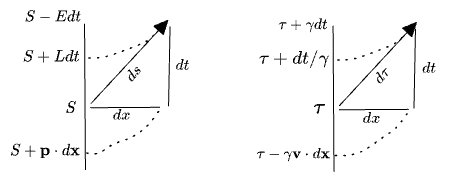
We can visualize this on a spacetime-diagram, using the fact that hyperbolae intersecting the axis at represent the set of points separated from the origin by a proper time . Then we can decompose an infinitesimal path element into two independent contributions to from and . We will take to simplify the visualization. We get:
In the left diagram the values are given in units of action; on the right they are in units of proper time . The action-units are more interpretable. We see that action is generally decreasing, being .
is the “action cost” due to the passage of time alone, as if the particle was at rest. The contribution is negative: .
as the “action cost” of the particle’s motion, with a positive contribution .
is the combination of the two. The total decrease in is smaller in magnitude than it would be for a particle at rest over the same time frame, , as it is offset by the contribution from the momentum.
In other words: if we start with , we see that the rest energy represents the “action per unit time” in the rest frame. In any other frame, the “action per unit time” is , which we can decompose into a contribution from time (in that frame) itself proportional to in that frame, and one from the motion of the object proportional to .
The E-L equations, which are mostly simply seen as a or , representing how a particle which is facing a spatial region of greater action-per-time (energy )—due to some interaction which couples it to the -per-time of other systems—will necessarily trade away some velocity, changing its Lorentz frame, so as to reduce its action-per-space (momentum ) to maintain the E-L condition.
Furthermore the proper time is just related to the arc length of the path: . So is, almost equivalently, measuring the arc-lengths of world-lines. Compare to a normal non-Minkowski arc-length:
These observations—when I found them, piqued by a stray comment from a professor—were the physical interpretations of I had been looking for. Circa 2011 this was nowhere to be found on Wikipedia, and never came up in any undergraduate courses, which probably seeded the frustration that has led to my writing all this down over a decade later. Maybe I should have learned more GR.
In this post I’ve started from Newton and then reached the “arc length” interpretation through a few derivations and a dose of special relativity. The better pedagogical derivation may be to assert the “arc length of a world line” as the underlying truth—starting with special relativity and then deriving classical mechanics from there might be more satisfactory.
V. to Euler-Lagrange, infinitesimally
We’ll now return to the question of deriving E-L from to look for another way down the ladder of abstraction.
The usual derivation of the Euler-Lagrange equations imagines varying a path and showing that the variation induced in is:
The first term is essentially our , but is taken to be zero by hypothesis. No terms appear because the endpoint times are considered fixed. Both of these obscure the physical nature of ! We’ve already established that the “endpoints are fixed” is unnecessary; the actual condition is that the action reduces to a function like of its endpoints, which I find more enlightening.
But the Euler-Lagrange equations are only a local differential equation, and should therefore follow from a local “stationary-action” principle, without any need to refer to a whole path or to any fixed endpoints.
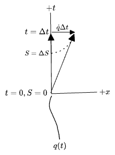
Suppose we have a path up to the point , at which point it has velocity and Lagrangian , and the action of the path so far is just .
Over the next time interval of size , if the path continued at its current velocity, then the action will update to like this:
The full update to the “state” will consist of:
The first few of these are straightforward.
picks up a contribution from ticking up at the current rate of action-per-time , and then secondly from changing over the interval . This latter contribution to is “second order” in , as the full effect of is only realized at the end of the interval. We will approximate it by its value at the midpoint of the interval, indicated with an overline , so as to express it as a first-order term in the series of .
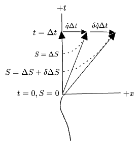
Now we consider a variation of the velocity at the beginning of the interval.
This will lead to a variation in along the interval, for a total variation at the end of the interval of . Either the velocity or position variation could be imagined to “cause” the other, but I prefer taking the velocity as independent—I like to think of all dynamics as producing changes in Lorentz frames, i.e. velocities, with the actual motion ensuing only from time-evolution.
Visually:
Note that a variation alters in the opposite direction of time-evolution. Since and , increasing brings about an increase in the value of , whereas pure time-evolution would make more negative.
Applying this variation then affects the state update occuring over the interval . We use for un-varied effect of time-evolution, and for everything resulting from this new variation in . We assume the velocity remains constant at the new value to first order. Then we have:
The final line for was the goal of this calculation. We find one variation due to the immediate change to which applies immediately, and is proportional to the initial momentum, and a second-order term which we approximate by its value at the midpoint.
Now that we’ve applied or , we ask: what condition on makes this vanish? Apparently , but there’s an extra , and those two derivatives aren’t evaluated in the same place. We can fix both of these by replacing
Then for we have:
And the Euler-Lagrange equation appears.
But the condition is not "". Instead our infinitesimal stationary-action principle has to say: when the E-L equations are satisfied, then the effect of an infinitesimal variation on must be equal to at the endpoint. But this is just the term as in the differential .
The standard “stationary-action principle” obscures all of this. You can’t make the infinitesimal argument with fixed endpoints; yet it is actually more intuitive. The standard argument with fixed endpoints uses a number of unnecessary hypotheses which are really besides the point, and misleading as to the physical content of the theory.
VI. and Legendre Transforms
One is usually introduced to the Hamiltonian as the Legendre transform of the Lagrangian; an explanation which sheds almost no light.
The are often omitted, which is permissible for convex functions—in that case, the meaning of the Legendre transform is
The explicit meaning of the Legendre transform is to invert the first derivative w.r.t. a single variable; hence expresses reparameterized by the value and expresses but reparameterized by . But the Legendre transform is not quite equal to the function with derivative is inverted; instead there is an extra which has the effect of making the transformation its own inverse, and of making it equivalent to integration by parts:
It turns out we can derive this relationship in another way, which I found somewhat clarifying. We imagine starting with defined in terms of a Lagrangian function which does not “know about” the relationship between ; they are effectively independent variables.
Then we enforce as a constraint, using a Lagrange multiplier, which will be a function of time :
We’ll call the inner function on the right the “expanded” action, which is a function of three variables before extremization:
Then a stationary-action variation of on is equivalent to the variation of all three of on . We can in principle perform these variations in any order. If we extremize w.r.t. all three variables:
We get that our multiplier is simply equal to the momentum , and an E-L equation, and we get the original constraint back. Inserting all of these results back into would just gives us the same extremal action as we would have gotten with the original action.
If instead we perform the variation first, we will get only the condition that the multiplier is just the momentum: . If we plug this back into we get:
Here .
But this is just the condition in the definition of the Hamiltonian; hence we can write:
This we can call the “Hamiltonian Lagrangian”—it is a two-variable functional. The extremization w.r.t. has allowed us to treat as an independent variable.
Extremization of w.r.t. both of will give the same extremal path as extremization of the original , but when we write this in terms of we get Hamilton’s equations as our “Euler-Lagrange equations”:
Furthermore, the extremization of w.r.t. only amounts to the Legendre transform of back into :
Mostly these just feel like tricks, but I do think they shed a little light—it’s helpful to distinguish and in particular.
We’ve used two particular “gestures” in this derivation:
First, we’ve re-expressed a Lagrange-multiplier problem as a pair of Legendre transforms by rewriting the original function in terms of a new variable , i.e. . Then the first Legendre-transform reparameterizes by the multiplier variable , the second by the constraint value . In the present problem, "" is the fairly trivial , but note that is not completely trivial if viewed as a function of , as it would be if we discretized the problem. Then the pair of Legendres are and , but we could also see these as Legendre transforms on itself: (omitting in the third term because it is no longer independent of .)
Second, we have taken an optimization problem (here over ), partially extremized it (w.r.t. only , or and ), and then plugged the result back in to arrive a “transformed” function with its own physical interpretation. This is useful! And it’s especially interesting to consider when some familiar expression can be seen as the result of this process being applied to a larger expression.
I wonder at this point if there is some way to transform along these same lines. It feels like there is some other way to look at in terms of Legendre transforms and Lagrange multipliers; one which ought to reduce it perhaps to nothing but constraint terms. The punch line of this argument still eludes me. I have written a few ideas here and then scratched them out; it isn’t clear right now. Well, one day.
This and this StackExchange answers were source for this section, and have more along these lines.
Conclusion
Here’s that map again:
So we’ve seen:
I: How to project Newton’s 2nd law to produce the Euler-Lagrange equations for a Lagrangian
II: How to integrate the E-L equations directly to get an action
III: How the E-L equations can be seen as the “curl-free” condition for the action as a function of its endpoint
IV: How the classical , with , arises from special relativity
V: How to derive the equations by requiring that over an infinitesimal interval rather than “looking into the future”
VI: How to arrive at the Hamiltonian , and the “Hamiltonian action”, by a straightforward reparameterization of .
III and VI are admittedly sketchy: the right physical condition that would lead to the curl-free condition eludes me, and VI doesn’t really seem to say anything. But they are, I think, stabs in the right direction—reducing the arbitrary operations we learn in mechanics class to be implementations of familiar operations.
The line marked , by the way, stands for “Legendre transform”. I have taken to privately calling this the “-transform” in light of the connection to Lagrange multipliers.
These, then, were the “missing derivations” from mechanics class—the arguments which would have satisfied my discontent, way back when. I’m not even in the field anymore, but I’ve had these questions bookmarked in my brain for years now, eating up some amount of working memory. Hopefully they can be of some help to someone else.
Were I ever to write a textbook on this material, I probably would not use my argument I or II. But I would cover special-relativity first, and then use relativity, IV, to justify a fully-fleshed-out version of III, the curl-free condition. The stationariness of the path could be mentioned only in passing—that can wait for some advanced quantum course.
The greatest advantage of a reorganization of material is that it may let you leave whole concepts and names in the dustbin. “Lagrangian” and “Hamiltonian” probably aren’t going anywhere, but perhaps we could do without variational derivatives and even without “Legendre”. The other major advantage is that it may let you teach the same material at a lower level of sophistication. The action is extremely important—it is emphasized throughout pop-sci books like Feynman’s Q.E.D., for example!—and yet it is relegated to the shelf of obscure machinery rather than being recognized as simply the length of a worldline. To dispel the obscurity around “action” makes the whole field more accessible, and will help to compress the body of knowledge of physics even for its practitioners—worthy goals, surely.