Dividing Vectors?
Table of Contents
Vector Division
I went to a lot of effort to justify the two multiplication operations
It is even more unusual to consider “vector division” at all. But I have a strong suspicion it will be useful as we go on to develop linear algebra along these lines, so we’re going to try to make it work.
In one dimension we were able to define a (nonstandard) division of vectors that worked exactly like division of numbers:
This gave a scalar, telling us “how many copies of
In 2D we immediately run into problems. The first is that we have three separate notions of “multiplication” to invert:
Note the three scalars appearing here—
Division 1: Projection as Scalar Division
We’ll take on
- We could treat this like “dividing by zero”, i.e. by forbidding it; assigning vectors to the class of forbidden denominators.
- We could expand the type of thing "
" is to include solutions for any pair of vectors. - We could define the division
to only divide the parallel parts of the vectors, i.e. giving . This is simple enough, but it would mean that our division operation is no longer a strict “inverse” of scalar multiplication.
This operation will be useful, so I won’t choose option (1). Option (2) is interesting but broadens the question considerably; we’ll return to it later on.
As a definition for the “division” of two vectors, I’ll choose option (3). Division of two vectors will be defined to be the division of their parallel components:
We will call this “scalar division (of vectors)” because it produces a scalar. Apparently, it is nothing but another way of writing a “projection”.
This notation:
- reduces to regular division for one-dimensional vectors
- is clearly dimensionless, because it looks like dividing one thing with vectorial units by another
- is undefined if
is the zero vector, just like regular division - is zero if
is perpendicular to .
Here I have introduced a convention which I have come to like: fraction notations like
Using this notation, we can easily decompose one vector into its projection and rejection by another:
If we are taking for granted a metric with which to define the lengths of vectors, this division operation is just an alias for3
Both the top and bottom of this fraction are length-dependent quantities, but the division-projection itself is a dimensionless scalar. Can it be defined in the absence of a scalar product?
To dip into some language we haven’t introduced yet: I believe the answer is that a metric is required, but a scalar product is not. The above is the action of certain covector we’ll call "
- an inner product, so we can define
- a metric
, with which to “lower” the index of . Then my . - or, a privileged basis including
, along with the constraint that for all basis vectors except for .
In the present treatment I am not concerned with spaces lacking a scalar product, so we’ll ignore these questions.
In fact, this division operation seems in many ways to be a more natural operation between two vectors than the scalar product itself. We can think of
Division 2: Dot and Cross Division
Next we come to
More importantly, there can now be, rather than zero solutions for
In each diagram below,
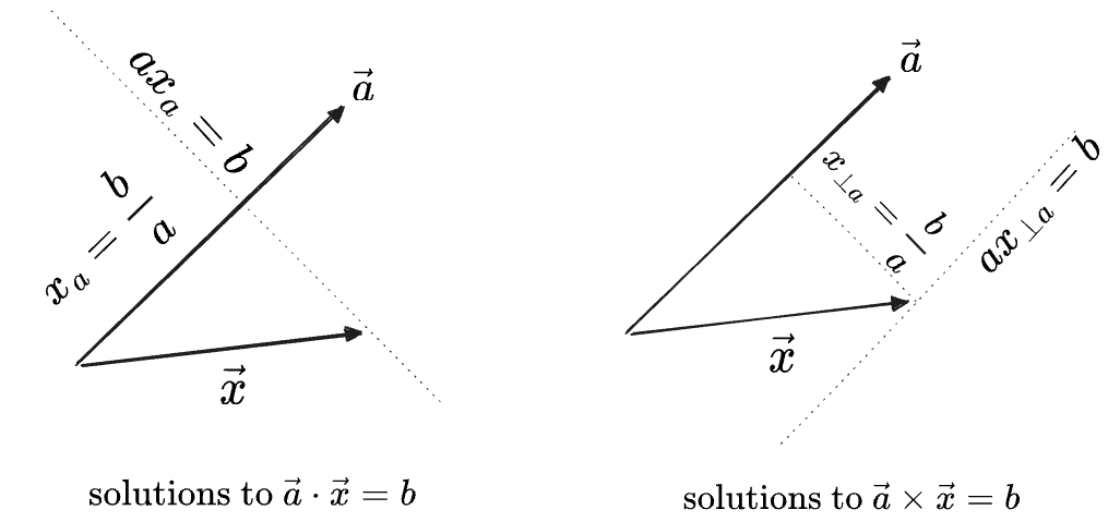
On the left the line of solutions is perpendicular to
We therefore have to make a choice in how we define these divisions:
-
We could skip these, treating them as undefined.
-
We could define the inverses of either product to give the entire set of solutions, i.e. the “preimage” of
. We’d get: - For
, we choose - For
, we choose
Note that these sets, being lines, are one-dimensional vector spaces themselves. We could also write these with the “constant” term factored out of the set, or even more succinctly in the “line” notation
from above: - For
-
We define the inverse of both products to be, not the set of all solutions as in (2), but the function of
which gives any element of that set, like this: - For
, we get - For
, we get
- For
-
We define the inverse of the products to be the “simplest” value from the set in (2), which is the value for
in (3), like this: - We choose the principal value of
for to be the vector parallel to which satisfies the equation, i.e. . - We choose the principal value
for to be perpendicular to in the direction which gives the correct sign for the cross product; this is . Thinking ahead to three dimensions, even this won’t even be enough: there will be an entire plane of vectors satisfying . We’ll solve this by changing the definition of , though.
- We choose the principal value of
Option (1)—just don’t do this—is standard, but I’m going to try to make the others work.
We will take (2) and (3) together as the same operation—which of the “set” or “an element of the set” is meant will be made clear from the context. These will be our first two examples of “generalized inverses”—multi-valued functions which arise as the inverses of forgetful operations. Our general rule will be to use
In each case the returned value is what would go in the “missing slot” of the product.
We can write an expression which treats this like a set:
Or we can replace the expression with a
We will always use Greek letters for the parameters brought in by generalized inverses, particularly
Then for (4), following the previous choice of
At the present level of abstraction the two placements for the
For
Note that using
Systems of Equations
As an example of the how one might use these inverses, we’ll try to solve a system of two linear equations:
We can rewrite this as two dot products with a single vector
Then the generalized inverses of these two dot products correspond to two lines. The overall solution is their intersection:
Here is the solution to one such system:
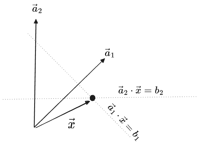
Apparently:
- if
and are parallel, and , then the two lines are the same and there are infinitely many solutions—the full set is given by either gen. inverse on its own. - if
and are parallel, but the two constants aren’t equal, there are zero solutions—parallel lines never intersect. - if they aren’t parallel then there is exactly one solution; the intersection of the lines.
To check if the two lines are parallel we simply see if
Then to find the solution for (3), we need to find the intersection of the two lines. We can find this by plugging one generalized inverse into the other constraint and then using algebra:
Here we’ve used
This is an explicit solution for
These are standard calculations, but this method has the advantage of being almost entirely algebraic. We haven’t even needed to use the word “matrix” or “determinant”. But it will turn out to be a great simplification to think of solutions to systems of equations as the intersection of row-solutions, especially in the case of underdetermined systems (our case 1 above). We will see much more of this kind of thing later on.
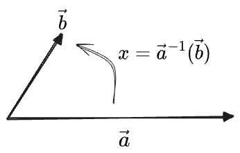
Division 3: Operator Inverses
In the discussion of scalar division, we punted on the idea of expanding the space of solutions to allow for a full inverse of “regular scalar multiplication”
What is needed is a “full inverse”
Of course, in this case it will no longer be “scalar multiplication”, the result won’t be a scalar. We might think to consider solutions within the space of 2x2 matrices, which I’ll write as
Only two of the four components of
One way is to look at the expression for a full “decomposition of a vector”
and ask if we can factor this entire expression as something that operates on
Here
The object in parentheses is an inverse of “scalar multiplication”:
If
It amounts to following choices for the unspecified components:
This is a full inverse within the smaller space of 2x2 matrices whose actions are invariant with respect to rotations of the space, that is, those matrices
This limitation feels acceptable, as “respecting rotations” was one of the principles we used to come up with our multiplication operations in the first place. So we’ll commit, and our definition of the “full inverse” of scalar multiplication will be:
Here I’ve notated this as a “function”
Using the
which acts exactly like the division of two complex numbers:
We can follow the lead of the complex operation and write our vector inverse as a matrix exponential, which looks strange the first time you see it but simply stands for its power series:
In the above we used
Note that while we started only with a
Division 4: Geometric Division
Now we bring together a few of the strands we’ve followed so far.
In the previous post we tentatively combined the dot and cross products of a pair of vectors into a single vector in a new vector space, called the geometric product:
Additinally, we established above that the inverses of the dot and cross product each determine one of the target vectors only up to a line (in 2D). This implies that if we simultaneously knew the values of
This implies that, if we were somehow handed a specific value in the geometric-product space of
and we can also define an inverse with respect to the first argument,
Now, suppose the specific geometric-product-vector we were handed was exactly
The above is conspicuously similar to the “operator inverse” or “matrix division” just discussed:
Both are true inverses. The difference is whether the inverse operation is applied to
except that in the present situation, it is as if the terms
Can we unify these two constructs? One way would be to:
- identify
with the geometric product , where is the metric-dependent “inverse vector” we touched on earlier. - identify
with and with - identify the action of a geometric product on a vector as being that of matrix multiplication by the basis matrices
.
But this feels tenuous. I can’t see a clear path forward. I am not comfortable simply saying these are the same thing, even if it works in this instance. We can apparently map geometric-product-vectors to superpositions of
Recap
To recap, we have come up with inverses for three different multiplication operations:
- Scalar multiplication
. We define only a principal value, “scalar division”, as , and this can fail to exist if the two vectors are perpendicular, akin to dividing by zero. - The dot product
, for which we define a generalized inverse and a principal value , which always exists unless . - The cross product
, with a generalized inverse and a principal value , which always exists unless . - More experimentally, an inverse of multiplication
which is an operator or 2x2 matrix in the subspace generated by . I’ve chosen to write this . - An inverse of the geometric product
, whose value is the intersection of the two constraints represented by that product:
None of these are conventional notations, though the “geometric product” definition comes close to that used in “geometric algebra”.
Ultimately, the test of whether these notations are wise choices wil be:
- are they algebraically self-consistent?
- or are they, at least, easy enough to use accurately that a user doesn’t mind their inconsistencies?
- are they useful?
The human mind can get used to a lot of caveats. (We become accustomed to many in the course of our educations.) So even a notation with a lot of weird loopholes should not be too hard to work with, given sufficient practice. But it has to be worth the effort.
For more on division notations, see my dedicated post on Division, where I try to make sense of the matrix inverse and other operations in terms similar to these ones.
With that we conclude our discussion of two-dimensional vectors. In next post, if I ever get around to writing it, we’ll take on the case of 3-or-more dimensions, where, hopefully, all this preparatory work will start to show its power.
-
To be well-moored in reality is very important for one’s sanity in the long run. And it helps to avoid spending too much of one’s attention on useless things, such as one’s grievances with one’s high school math education. ↩
-
This operation has a certain similarity to “floor division”, i.e. like
, with the component as the “remainder”. Another notation which suggests itself is then a double slash , which is how floor division is notated in many programming languages. Or a unicode double-slash could be used, , or a fraction with a double bar line which I have no way to represent here. We could further use a modulo sign to represent the “remainder”, . While interesting, I’ll stick with the regular division notation in this post. ↩ -
Note that
is not equivalent to , despite it seeming like “dividing the parallel components of vectors” should be indifferent to which vector we project onto the other. ↩ -
Another notation which comes to mind is to use
for an inverse of the dot product, because it looks like a fraction with dots on the top and bottom: . We can hack a version for , too: . I don’t have full LateX support here, so that’s written ~\substack{\small\times \\ \_\_ \\ \small\times}~. I don’t think it’s too bad! We could also go in the “floor division” direction as mentioned earlier. But I think the fraction notation will be sufficient. ↩ -
The intersection appearing in the geometric inverse looks suspicious. But this is really exactly how a matrix inverse works: if you view
as a set of constraints , the solution is . Indeed, the geometric product could simply be written as a matrix equation. ↩
Comments
(via Bluesky)