Generalizing Division
Table of Contents
- Introduction
- Scalar / Scalar
- Scalar / Vector
- Vector / Vector
- Vector / Matrix I: Orthogonal Matrices
- Vector / Matrix II: Non-orthogonal Matrices
- Closing Remarks
Introduction
The opposite of multiplication is division, right?
This series of posts will attempt to develop a non-standard notation for linear and exterior algebra by making extensive use of “division”. I’m not sure if this is actually a good idea, so the reader should beware.
Scalar / Scalar
If
There are three cases:
Case 1:
Case 2: … unless
Case 3: … unless
Easy. Now let’s talk about vectors.
Scalar / Vector
If
Three cases again:1
- No solution, unless we’re in one dimension. The equation fixes the component of
onto to be , but we’re free to add any perpendicular vector without changing the answer. - … unless
is zero, in which case even there are no solutions. - … unless
is also zero, in which case any -vector is a solution.
Note (2) and (3) are the same special cases as in scalar division.
For (1), the set of solutions is a “generalized inverse” of the function “dot product with a vector
This can be thought of in a few ways:
- a) as a set of solutions
- b) or as a “standard” solution
plus any single element from the orthogonal subspace - c) or as a function to solutions, depending on the choice of element in the orthogonal subspace:
Of these, (a) is most commonly seen, but in this post I’ll prefer (c).
My preferred notation will be as follows. The full inverse be represented by
This full solution will be called either a “general solution” or a “generalized inverse”. The “standard” term might also be called the “principal value” or “adjoint”.
The “division” notation is the main point of all this. This “generalized inverse” with a “division” for a “standard part”, will be our 4th “prototype” case of division:
Case 4: Division gives a solution only up to the addition of a term which multiplies to zero, for whatever definition of “multiplies” we’re currently using.
This is non-standard, reader beware, but my aim is to take it as far as I can, as a way of unifying what would otherwise be a number of distinct concepts.
How should “division by a vector” work, then? It is apparently equivalent to
The two copies of
and
But we’ll want to be careful about assuming these act like regular fractions in any other ways—these “fractions” will only have the specific properties we name.
We’ll take on the case of vectors not parallel to
The standard part
The remainder
In 2D we can span the space
Note that I’ve used
In
I’ll use the symbol
If the same basis is used for
This demonstrates that the “generalized inverse” acts like a combination of:
- regular division on the single dimension
, with solution . - zero divided by zero on the other
dimensions, with the free parameter representing “any solution” to these divisions.
This is rather imprecise, though:
Before we move on, I’ll note one common example that works like this: the integral
The constant function
Vector / Vector
If
Three basic cases:
- If
and are parallel, then is the ratio between their lengths. So if , then . Easy. - … unless
, in which case there’s no solution. - … unless
, in which case any is a solution.
But if
Case 5: Division can be defined to give a standard part but is not a “generalized inverse” of multiplication. Instead a remainder is left over.
The remainder case is exactly what occurs for scalar division on integers. If in our original scalar example
We will want to think of the remainder here as being “part” of
Returning to the case of vectors,
Evidently the parallel part can be seen as the “best” answer for “division”, with the perpendicular part the “remainder”.
Rather than a floor symbol
In the scalar-over-vector case, multiplying by
This will be a general pattern: division-and-multiplication produce a projection. Apparently we can sort of treat this like a fraction and move the multiplied vector into the numerator, but this will only work for vectors parallel to the denominator.
In two dimensions we can do the same for the rejection term, letting us write the decomposition of the whole vector
In higher dimensions we’ll have to use a matrix in place of
You can think of division-as-projection as measuring “the number of times
The rule “division means projection” turns out to be exactly what is needed to interpret a standard derivative
Here
This does not work for partial deriatives
I introduced the projection notation as a natural extension of “division with remainder”, but there are a couple of other ways of looking at it.
The first is to expand
This is clearly now a case of “dividing by zero”. Furthermore these are
Secondly, we could expand the space in which
Case 6: Division is defined as an exact inverse, but within a larger space of solutions.
Of course this can get out of hand—you could in principle expand the space to anything. The trick is to expand it as little as possible while still getting a division operation that’s well-defined.
For the present example, if we let
The equation
but this is apparently more degrees of freedom than are actually needed. Two will do, and an obvious choice is to write
which is a true inverse of multiplication:
This is not the only choice of two “basis” matrices out of which to construct the inverse, but these are particularly nice ones. If we call
The first term is obviously the projection analogous to
In more than two dimensions, any matrix which rotates
One can take this line of thinking much further, but we’ll turn back.
Now, if we can decompose a vector into a projection and rejection by dividing and multiplying,
we can surely decompose it into an orthonormal basis in the same fashion:
This will work even if the basis vectors are not unit-length, since the lengths divide out, but it won’t work if they’re non-orthogonal.
The above expression looks something like a single “division and multiplication” on the entire basis at once, i.e.
But to assign a meaning to this in generality we need the matrix inverse, which brings us to the next section.
Vector / Matrix I: Orthogonal Matrices
We’ve bumped into the matrix inverse three times already:
- when we wanted to put coordinates on the
term in the generalized inverse - when “expanding the space of solutions” of
to get - just now when considering the components of a vector
in an arbitrary basis:
The third case is the simplest, so let’s go in with that in mind. And I’ll start by considering the simplest case of a matrix of
Invertible Matrices
For now,
The scalar and vector components of
This means we can immediately write down the matrix inverse
The matrix shown is therefore the inverse
That is the simplest case: the matrix is perfectly invertible, so its “generalized inverse”
We can also convert the inverse-vectors into regular vectors:
The denominators of these fractions are the diagonal elements of
so we can also write
Thus we have
Before we move on to non-orthogonal columns, let’s look at how the cases of (2) “division by zero” and (3) “zero-over-zero” arise for matrices.
Overdetermined Matrices
“Dividing by zero” is most easily seen in the extremely simple example of a diagonal matrix which has only
This gives
which can of course be solved, and
which can’t be solved in general, unless the
(This is also the general case: any matrix can be transformed into this form via a “singular value decomposition”, although the vectors
When talking about matrices this case is called “overdetermined”, and it arises either when
We can view the overdetermined case in a few equivalent ways:
represents distinct equations in unknowns (which is the source of the word “overdetermined”) - Or,
is not in the span of the columns of and therefore cannot be assigned “coordinates” in the basis of its columns. - Or, the
rows of , each of which is a constraint of the form , amount to contradictory constraints on the vector .
But of course we’ll still try to define a “standard part” of the inverse in the overdetermined case. We’ll treat it like “division with a remainder” and define a “fraction”
For the diagonal example this is simply:
The “rejection” or “remainder” term
In the above example I’ve set
In all we have:
I’ve used two different symbols
The following diagram sketches the full picture:

It’s just as easy to define the standard part of the inverse for the earlier example of a matrix of “orthogonal basis vectors”. If the first
This again inverts each basis vector separately
and we can write this in “numerator form” as shown earlier, which is the pseudoinverse:
The “standard part” notation is conveniently ignoring the zeros in
Given this we can easily write the rejection/remainder/cokernel term as well; it is the term usually appearing in the pseudoinverse equation:
Underdetermined Matrices
What about the case of “zero divided by zero”? This typically occurs when
An equivalent case can arise for square matrices when the rank is less than
- The span of
‘s columns is less than the full space, but is in this span. - The row-constraints
are duplicated constraints on (rather that being inconsistent with each other.)
In either case an inverse will exist, but there will only be “free parameters” (akin to
The simplest underdetermined case is a diagonal matrix:
It will be easier to write these in block notation, so the above is equivalent to:
The “standard part” of the inverse is clearly
and the generalized inverse is
which is just the component representation of
The “mixed case” can be seen on the simple example of a diagonal matrix, where it looks like
Here
The underdetermined case on “orthogonal basis vectors” works exactly the same as the diagonal case, so I’ll skip it and we’ll move on to non-orthogonal matrices.
Vector / Matrix II: Non-orthogonal Matrices
I’ll now assume that the columns of
Invertible Matrices
Conceptually, the simplest way to understand the general matrix inverse makes use of the wedge product
We begin by writing out the above matrix multiplication in a way that suggests an interpretation as “the coordinates of
We can then “solve for” any single
This can also be seen as the “
Of course this construction is zero if
For any other column
At this point the left and right sides are both
This is “Cramer’s rule” in a slightly esoteric notation. The denominator is equal to the determinant of
The above expression can be interpreted for now as a ratio of two scalar areas, but is in fact a “standard part” of a division of two
Then the volume divides out, and we can rewrite
The matrix inverse “standard part” is therefore:
This expression is analogous to
We can also identify
as the “dual basis vector” to
I don’t find the final inverse expression to be very enlightening, though. The clearest expression is
which says: to find the component of
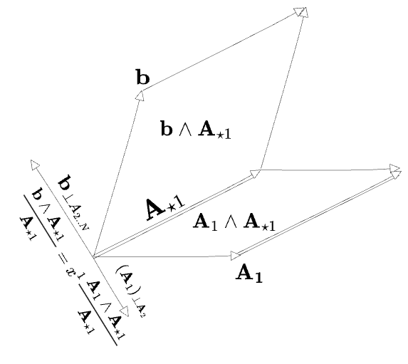
This can be understood visually with the aid of the diagams following. I’ll consider

As can be seen by studying this diagram, it is not the case that
If we had first determined
It is somewhat surprising to me that the two requirements ”
The next diagram depicts the same argument in terms of areas:
I’ve now written
So we’ve found that the general case of the matrix inverse has a standard part that is not simply
but the Cramer expression (using
This, by the way, is exactly the same as the distinction between a total derivative
This suggests first that the act of taking a “partial derivative” with respect to
The denominator will clearly give a Jacobian determinant, but I’m not sure what to make of the numerator. I suppose it will turn out to be
Non-Invertible Matrices
What about the cases of over- or under-determined matrices? In either case we know from the preceding section that
where
We can also see this as starting from the view of
and then wedging both sides of this expression with only
In either case the generalized inverse will then take
We can go a little further and use Cramer’s rule to write an explicit basis on the subspace
lies in the subspace
The
which is clear enough, although not particularly useful.
The takeaway is that Cramer can be used for over/undetermined matrices by applying it only to some maximal set of
Something about this approach feels unsatisfying, though. If the original Cramer formula worked and let us define a standard part
then the Cramer denominators
It feels as though these zeroes could be “cancelled out” to produce the rank-
I’m not sure if this notion can be made precise. I think a better view might be to think of the Cramer formula in areas as a “reduced” description of the full matrix
I suppose the “diagonal” representation I’ve been using (which as noted can be seen as the SVD of the original matrix) might be a candidate, but that doesn’t feel quite like the thing I’m looking for. But this has gone on long enough, so let’s leave it for now.
Closing Remarks
In total we have toured the following things which look like “division”.
gave us scalar-over-scalar division: required a generalized inverse, which we could write as a scalar-over-vector division and a “free parameter”: , led to vector-over-vector-division as a notation for the projection , and also required a “remainder” led to vector-over-matrix division which could be identified with the “pseudoinverse”, and which required both “free parameters” and “remainders” in general. And we also saw how this could be expressed in terms of wedge powers as a Cramer type formula, in general written as .
Six “cases” came up:
- An exact solution
- Division by zero, which had no solution
- Zero-divided-by-zero, which permits any solution
- The free parameter, which was required when (2) or (3) red along some dimensions of the problem
- The remainder, which was required when (2) occurred along some dimensions of the problem
- And “moving to a larger space of solutions”, which we touched briefly when solving vector-over-vector division with rotations.
All of this is really preliminary work for a larger project—my aim at this point has been to get my thoughts in order. There are two issues in particular which I did not take on in this post:
- How complex numbers arise when diagonalizing matrices, which can be seen as an instance of “case 6”. I mostly avoided this by considering everything from the view of SVD, but in general it will be interesting to see how complex numbers arise when trying to invert purely-real systems.
- Matrices requiring Jordan Normal form. Whatever I once knew about this I have long since forgotten, but my understanding is that these too can be diagonalized by a “case 6”-type maneuver, but now by adding “dual numbers” with
to the number system.
That is surely enough for now, though. The next post in this series will be an attempt to express the basic constructs of exterior algebra as “divisions”; my hope is that some of these wind up appearing so elementary that they hardly deserve having their own names, but we’ll see.
-
For a thorough exploration of this kind of division, see my post on Elementary Linear Algebra. ↩
-
I am being fairly imprecise here by pretending vectors may be identified with their duals.
doesn’t, in fact, do anything to its row space; does. ↩
Comments
(via Bluesky)