The Entropy Function
Table of Contents
1. Interpreting Shannon
Here again is the “Shannon entropy” of a probability distribution
Its argument is a discrete probability distribution, which we represent as a vector, as a function of an argument, by its distribution, or by a random variables:
The square brackets
The simplest example is the entropy of a uniform distribution over the
We get
The formula also interpolates cleanly over non-uniform distributions
In the first post in this series, we saw that the entropy
The entropy may also be identified as “average decrease in log-probability per sample” of a sequence drawn from the distribution
We also saw that the same formula arises when taking the large-
which implies that the relative probability of observing a given set of counts
We can arrive at another characterization by noting that the entropy can be written as an expectation:
where the object
We can then express
which suggests we interpret the entropy either “average information required to specify a particular element” or as the “expected information gained by learning the exact value of a sample”.
2. Basic Properties
If we start with a single set
and then we divide it in two
the entropy, as measured in base-2 bits, goes up by
The same applies for any division into two:
For each block of weight
Therefore, dividing every block in two at once increases the total entropy by
If we interpret entropy as giving the information required to “address” or “label” the elements of the set, then dividing each element in two can be interpreted as saying: the new distribution
Likewise subdividing or “fine-graining” by another factor
Such a “fine-graining” is equivalent to replacing the distribution
which leads us to a general rule that entropies add over products:
Note this is the same as the behavior of a logarithm on numbers:
and the two laws coincide in the case of uniform distributions1:
We can go in the other direction to calculate the entropy of a coarse-graining or aggregating operation. For any distribution
So grouping
And grouping all
Note that the term subtracting in the above is exactly the (fraction occupied by the merged block)
Rearranging gives
in which we can read two the entropy of two equivalent algorithms:
- either we first select a block from an uneven distribution
, then select uniformly from within that block according to a - or, we select one element from a
distribution
Clearly we should be able to count or address a set of
3. Visualizing Shannon
Each term in the Shannon entropy has the form
whose graph looks like
That’s an odd shape, but it doesn’t mean much on its own. It is the product of
More informative is the graph of
It’s nearly a perfect circle, peaking at a value of
We can also visualize the entropy over all possible probability distributions on a three-element set. The three probabilities
Again we see that the entropy
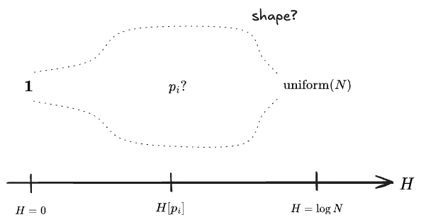
For more than three probabilities no direct visualization is possible. Instead, let us try to say something about the shape of the space and the range of entropies on it.
Within the space of all possible distributions
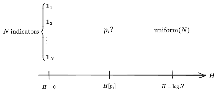
What happens in the middle? What fraction of all possible distributions have the given entropies? Certainly there are vastly more uneven distributions than either the indicators or the single uniform.
Let’s first try to take on a simpler problem by considering only distributions which can arise by grouping
Let’s play with a few, starting from the single partition
… but the three-way partitions quickly overtake the two-way ones, and of course there are a lot of these. The total number of partitions of a set of size
As it’s 2025, I can ask an AI to count them all in about two minutes.3 Here’s a visualization:
There’s a clear shape, peaking (the AI tells me) near
Returning to the first question: what if we did the same for the set of distributions on
Well: it’s a similar shape. Note the y-axis is not a log-scale in this one, as the whole region near 0 would go to
Before we move on, I want to register a couple of stray thoughts:
- I find the distinction between the entropy of partitions and distributions here to be suggestive. I suspect that entropy is more naturally defined on partitions: elements with
effectively don’t exist from the perspective of the entropy. All indicator distributions are the same thing, information-wise (it’s the underlying set which is different). I’ll have to think on this. - The first visualization acquires its shape only from the integer-partitions with the highest set-partition multiplicities. It might make more sense to smooth this curve out, so as actually get a sense of the measures in the neighborhood of each
value. - I don’t think a “uniform measure” makes sense on the space of real-valued probability distributions, so the second visualization just given is probably not very meaningful. It might actually make sense to use the entropy itself as the measure on that space, as
is the asymptotic measure a distribution arising from samples from a uniform, by the third argument from the previous post in this series. But I won’t try to take that on now.
4. Entropy vs. Variance
Here’s one visualization of some entropies. Now—unlike all the earlier examples—we will associate the indices
Playing with this, we can observe a few things:
- the uniform distribution has the highest possible entropy for a given number of bins.
- all of the indicator/delta-function distributions have entropy zero (and variance zero).
- in general, entropy will be low for very peaked distributions, and high for spread-out ones. In this respect it is similar to the variance.
- but the entropy is unchanged when the cells are shuffled, while the variance will tend to vary a lot.
(Note that you can put in unnormalized distributions, but they will be normalized before calculating the stats.)
Both the entropy and variance characterize the “uncertainty” or “spread-out-ness” of a distribution. Both are zero for an indicator and large for a uniform distribution—but the entropy attains its highest possible value on a uniform, while it’s easy to make the variance even larger by creating something bimodal. (If you click the “Beta” button enough times you’ll get something bimodal, or you can draw your own.)
What’s the difference?
We’ll write the entropy of a r.v.
Despite this notation, the entropy does not depend on the value of
Yet if we plot the two against each other for a few typical distributions, they appear to be closely related:
(The normals and betas here are discretized, rather than continuous distributions. We’ll address the entropy of continuous distributions another time.)
What’s going on?
Let’s investigate further. Here are a family of normal distributions centered on
We see a clear pattern, which interpolates between the nearly-indicator-like
Here now are a family of
Again wee see entropies and variances which decreasing together.
But all of these distributions have been approximately normal; guided by our first widget we probably need to be looking at more spread-out distributions.
Let’s try a contrived scenario: you flip a coin of unknown
If we take our prior on
which looks like
There’s still a tight relationship between entropy and variance, but now it goes the other way.
The difference seems to be that these new distributions are bimodal.
Apparently we can change the variance of a distribution quite freely without affecting the entropy, simply by shuffling it to be more or less spread out.
Then if find can find some family of distributions with equal variances, then their entropies must vary.
Let’s try it. In the following I started with a
The point is: entropy and variance are closely related for unimodal distributions, but not in general. They can vary independently, though it can take some pretty contrived distributions to demonstrate it.
Further investigation sheds some light. Apparently, there exists a series expansion for the Shannon entropy in terms of the cumulants of a distribution, which are certain functions
This was surprising to me, since the Shannon entropy doesn’t depend on the values taken by the R.V.
Interactive visualizations for this post were authored with D3.js in Typescript, embedded in a Marimo (Python) notebook via anywidget with considerable help from Claude Code, and then manually ported into React components to be consumed by Astro, which builds this site. The simpler plots were built with Bokeh and exported as HTML. Mostly this was a pain and I wouldn’t do it this way again, but it is worth noting that Claude is excellent at one-off D3-type visualizations.
-
I find this law to be very suggestive—entropy appears to act like a generalization of “logarithms” to the large space of distributions, where we identify the uniform distributions with the original space of numbers themselves. We can follow the analogy in the other direction to interpret logarithms as an “information” function in all cases. Aren’t integers, after all, just an abstract “count” of something? ↩
-
One can also derive the formula for
in the first place by asserting a handful of properties like continuity, the logarithm-like property on product distributions, and the equivalence of the two selection processes just given; see wiki. ↩ -
Here’s the chat, including a lot of extra—and impressive—analysis. ↩
-
In statistical mechanics, the logarithm of the partition function,
, turns out to be a cumulant generating function, which is one way of explaining its many surprising properties. ↩
Comments
(via Bluesky)