Observe the rules of variances and standard deviations:
Compare with the vector inner product and norm:
Evidently acts just like a squared norm , and a covariance acts just like an inner product.
This one notices right away, probably on one’s first encounter with random variables. But we lack the equipment to explain how this might be so. It is filed away as a curiosity.
Let us ground this “vectorial intuition” for probability distributions, then. In what sense is a probability distribution a vector?
I will be a little technical, so as to untangle what might otherwise get confused. (I was myself confused.)
Suppose we have an underlying sample space . The set of events may well be non-numeric: the faces of die, playing cards, or the outcomes of a sporting event or election. Or they might be inherently numeric: the temperature on a given day, the number of deaths or births, etc. In either case we somehow come by a probability measure over this space: perhaps we invoke the “principle of indifference” for the die, or we forecast a distribution of outcomes for a soccer match. In any case we assign weights to the elements of such that . But note that, at this point, we can not define a “mean” or “variance” of ; the events themselves may not have any inherent numeric value (though they may if is a set of numbers).
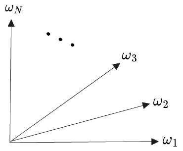
Now we create a random variable, which assigns a real number in some subset to each event: . The original distribution now pushes forward to a measure on . We may now speak of a “probability distribution” over the numbers in —a dice roll may be described by a discrete uniform distribution over the set , some temperature measurement might be described by a normal distribution around some mean temperature , etc.
With this distribution (defined by the p.d.f. or measure ) we can now define expectations on , such as the variance of the random variable , or some other r.v. defined as a function of :
Or the covariance of two random variables:
(Here is a given as a function of the variable for simplicity.)
Now: it is the random variable (like ) which we will view as a vector. It is not the underlying probability measure or distribution (like , , , or ). I found this point confusing.
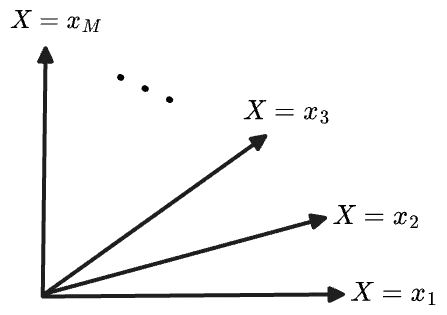
The requirement for a random variable to be a vector is that its second moment be finite: . This is exactly the condition of being “square integrable”, , for the function . This makes a member of an inner product space on with respect to the measure , with the mixed moment as the inner product:
Or we can regard as members of the space on itself, now with measure and a coordinate :
Or for two random variables defined directly on the underlying space:
At this point we have found the vector space in which a random variable is a vector. It is a Hilbert space of functions-over-something; exactly like the Hilbert space of functions with Fourier expansions, or of quantum mechanics.
But this is not the whole picture, because the inner product referred to above is not the covariance . And is the norm of but is not the variance, which would be .
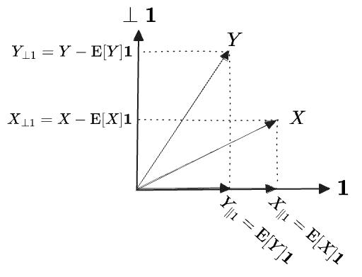
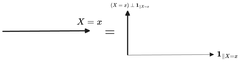
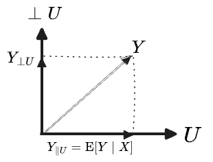
To get the covariance we have to compare, not the r.v.s themselves, but their rejections off the subspace of constant functions. The “constant functions” are all multiples of the unit constant function , which corresponds to the vector . (It’s a unit vector because its norm is 1, since our measure is a probability measure and integrates to , .) Then the expectation/mean is just the inner product with this unit vector:
Therefore the difference removes the component of along one particular unit vector:
The variance of is then the norm of ‘s component on the subspace perpendicular to , which I’ll shorthand as :
The standard deviation is a norm:
And the covariance between and is an inner product:
So: the covariance of two random variables is indeed an inner product on a vector space. Hence, all of its properties.
We can easily visualize this, too:
That’s the punchline. In hindsight it’s nearly trivial, but when one treats probability distributions as vectors it is usually in the context of vectors of samples , and I had a hard time connecting the probability-theory part of my brain to the functional-analysis part to see that was an inner product with the vector representing constant functions.
Sample Variance
Now I want to investigate a couple questions which came to mind during the discussion so far.
My first question is: what about sampling distributions?
Here the situation is: we observe values of the random variable . These are the genuine values of restricted to the points ; it is the choice of the points which is “random”. So we have:
From these samples we would like to characterize the underlying random variable , by e.g. its mean and variance.
These points define a a new random variable on a new sample space which is just the set , with a discrete uniform with weight . (We’ll assume all samples are distinct.)
Distributions on the discrete space are just vectors in , so can define a new space with the uniform measure . Variance and covariance on this sample space can then be defined as inner products exactly as we did before (with the sample mean ):
Just as in the case of , we are removing the component of along the constant functions on and then computing an inner product on the remaining -dimensional subspace.
The factor enters as the discrete measure on the set .
But the latter expression is not the “sample variance”. Here we come to the matter of the factor in the sample variance, Bessel’s Correction. The “unbiased estimator” of the true variance of is:
It is straightforward to prove that is necessary to correctly estimate . We draw three vectors in the vector space over the sample space representing the data, the sample mean, and the true mean:
Here is the constant vector on the sampling space .
The differences of these vectors form a triangle:
And it must be a right triangle: the third vector is the hypotenuse of the right triangle formed by the first two, since is just the projection of onto , making perpendicular to and therefore to . Therefore the norms of these vectors obey a Pythagorean theorem:
Meanwhile the expectations of these norms in the original space may be determined from the properties of the variance:
The last of these is the expression in the sample variance: in expectation. Hence it is which estimates .1
But let us try to see why this might be true in terms of the inner product view from above.
To compute in requires we 1) project off , then 2) take a squared-norm.
To estimate from a sample , we 1) restrict to , 2) project off , 3) then take a squared-norm. This would have an identical if the operation “restrict-then-project” removed the same component as “reject” alone, but it doesn’t—we subtract , not .
If we happened to know the true mean , we could estimate the variance by , which would not be biased. This would be 1) projecting off , 2) then restricting to , then 3) computing a squared-norm.
The difference is the “commutator” of project-then-restrict as opposed to to restrict-then-project. Well, this is just , and its squared-norm is equal in expectation to . We fix this by changing to .
Is this illuminating? A little. I find it a bit clarifying to note that a sample variance is trying to approximate an inner product (potentially on an infinite space) by an inner product on a different space.
Exterior Products?
It is evident from the discussion above that the covariance matrix of a random vector is just the Gram matrix of its components after projecting off the constant components . That is:
One can also define a matrix between two random vectors as a Gram matrix with components .
A Gram matrix then has a “Gram determinant”, which usually comes up as a way of determinant of the components of are linearly independent. But for this purpose it’s overkill: an -way wedge product would suffice. The Gram determinant, in fact, is the squared-norm of the exterior product of vectors:
And the determinant of a two-vector Gram matrix is the inner product on the th exterior product space:
This raises the question: given that random variables are vectors in , what is the meaning of a wedge product of random variables?
The wedge product of random variables would—I believe—look like
since it needs to act on two separate copies of . The norm on this wedge power is:
If we restrict to first, the matrix becomes the covariance matrix of the vector and its norm is
which is a perfectly useful measure of linear independence, related to Pearson’s . But this is just the covariance matrix again.
… and here I find nowhere to go. I asked the AIs for help and they too turned up nothing. And exterior algebra gets complicated if is taken to be infinite-dimensional. Evidently, it is not that useful to take exterior powers of random-variables, perhaps because they have no particular geometric interpretation. So I’ll file it away.
Conditional Expectations
Another question. What, in vector space terms, is the meaning of the (surprisingly confusing) conditional expectation?
This, a bit surprisingly, is a random variable on the same space as and . It maps each distinct level set of to a single value
For the purposes of computing the conditional expectation, we may treat as having coordinates, as any other dimensions of variation will be marginalized-over anyway. So we have:
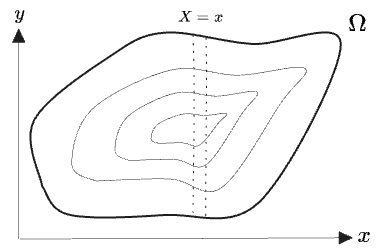
In the simplest case, and define distinct coordinates on :
I’ve depicted as a blobby shape, with contour lines suggesting a distribution on the space. A sample space need not have any “intrinsic” shape like this, as it’s just a set. But given two non-equal random variables , we can always increasing values of as an coordinate and then take as a y-coordinate to arrange the elements into some kind of blobby shape.
Note that and describe a random variable and distribution over the highlighted slice of only—this is a different space from the original . (And on its own is not really a thing, but could be perhaps defined as a function of which gives a random variable for each .)
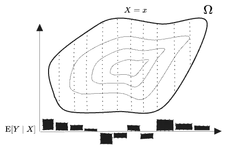
The conditional expectation then assigns, to each level set of , the value of on that level set. That is, it assigns values to all coordinates, but these values are constant over the level sets. A 3D graph is hard to draw, but since the values are constant in the direction anyway we can show them as bars off to the side:
(The values of shown are just made up here, and have no relation to the contours on . The point is only that this r.v. is constant on level sets of .)
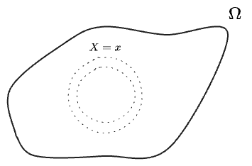
Note that, if for some reason our is best visualized in some other way, the sets of could easily have other shapes:
And, note that need not vary “orthogonally” to at all: it could simply be a function of itself, like , which would mean that it takes only one fixed value on each level set of .
Now I want to visualize exactly what is doing in terms of the vector space of random variables over . I’ll limit the rest of the discussion to finite vector spaces, to avoid the many technicalities which arise with conditional expectations for continuous spaces.
For a finite sample space of size , the r.v.s are elements of , so there is clearly a basis consisting of the indicators on each point of ; this is just the standard basis, but we’ll label them by their underlying point in . We can schematically depict the vector space:
Then the level sets of , for each of the distinct value in its image, are each a subspace of the overall space
where I’ve used thick lines to indicate that each subspace has dimension .
Each level-set subspace is obviously spanned by the indicators on its points. For example, if a specific value occurs at exactly 3 points, the is three dimensional and has a basis of three points’ indicators:
For any , there is a one-dimensional subspace where consisting of those vectors which are constant on the level set. Among these is the projection of the global constant vector onto this subspace, . The remaining dimensions of the subspace are orthogonal to this vector, . In terms of this decomposition, is:
Now, the conditional expectation is constant on every level set of , with value equal to the mean of on the level set. Therefore its value on that subspace is exactly the projection of onto :
The probability required to get has conveniently appeared as the squared-norm of .
The full conditional expectation must therefore be the projection of onto the sum subspace of all the vectors constant on each level set of :
The rejection is the vector of “fluctuations” in relative to . The two add to , of course:
Visualized:
Well, that’s satisfying.
It would be nice to give the subspace a special symbol, perhaps . But at a glance this reads like some kind of regular projection of , and would give just a one-dimensional vector. We would have to give some special semantic, similar to (my preferred symbol for vector projections), such that specifically leads to the just given. I doubt this construction would be much use outside of the context of random variables, anyway, as one usually does not have such a privileged basis of indicators on which to define “level sets” of a vector; it is obscured here but the entire idea of is defined w.r.t. the indicator basis in particular.
Anyway, the conditional expectation has been adequately elucidated. We won’t go near the infinite-dimensional case, but I’m sure it works about the same way.