Time Evolution
- (This post)
My aim in this post is to plot a simple course through elementary dynamical systems theory to arrive quickly at some of the basic elements which appear in physical theories like quantum mechanics. In learning physics we normally encounter many of these concepts only when we first need them, and rarely see clearly how generic they turn out to be. It should help to follow the story from the beginning—all we need is first-order ordinary differential equations.
Table of Contents
- Direct Integration
- Generating a Flow
- Higher Dimensions
- Three Views of Time Evolution
- Time-Ordered Exponentials
Direct Integration
Our subject will be the trajectory
In the simplest case of a constant velocity the trajectory is given by the integral
where
For
the trajectory is the general integral
where the integral sign stands for nothing more than the repeated application of the linearization
The integral expression must be equivalent to a Taylor Series where
We could generate the individual terms of this series by repeatedly expanding the previous integrand to first order:
This series is suggestive of the series expansion of an exponential
This expression is basically a general solution to time-translation, and could be evaluated term-by-term by substituting
The system specified by a velocity function
Generating a Flow
What if
The ODE
can be integrated to an awkward but general solution:
For example, if
which is readily solved (ignoring the absolute values, which add a wrinkle) to give
representing a trajectory which exponentially grows or decays, depending on the sign of
Calling the l.h.s. integral
If
This is not as nice an expression as the others, but it looks like something we can expand in a series. The inverse function theorem for the derivative will be useful: from the fact that
Evidently each derivative applies a factor of
With these, the series expansion is
and the last line looks like the series expansion of an exponential function whose argument is the “generator”
The strange-looking exponential here
and the time-evolution of the identity function
We might have been able to guess the form of the generator by observing that
which is suggestive of an ODE
Higher Dimensions
Next we ought to visit the
What happens? Well, nothing about the derivation in the previous section required one dimension, so we can quote the solution in the function representation:
and the time evolution of a trajectory is the same expression on the identity
Of interest is the simple case
and
so the general solution is simply
The corresponding 1D case
Exponential growth and decay, at once along different eigenvectors, e.g.:
Rotations, where two dimensions flow into each other while other dimensions do other things:
where
Shears, the simplest case of which is a nilpotent matrix leading to linear trajectories of varying speeds:
The effect is basically predicted by the series solution:
with
Transients of various kinds:
A general real matrix
- The dimension being sheared-into could have its own growth or decay rate:
Here, if
could be a pure rotation with then sheared into , causing to couple to the oscillation itself at a lag:
could be exponentially decaying, while shearing into , which will cause it to grow transiently and then level off:
- Multiple dimensions could shear into the same one, with various transient effects.
In general the classification scheme is:
- if the matrix is normal,
, then its eigenvectors are orthogonal, and its dynamics “factor” into distinct orthogonal dimensions with their own growth or decay, or into pairs of dimensions exhibiting rotations. Classifying eigenvalues suffices to characterize behavior. - if not, the eigenvectors are non-orthogonal and can feed transiently into each other.
- if furthermore the matrix is “defective”—it has a non-trivial Jordan Normal form, and fewer eigenvectors than dimensions—then polynomial-in-time terms like
appear.
For various reasons physical systems rarely exhibit these latter exotic behaviors, among them that these will tend to violate conservation laws, and that they are unstable w.r.t. perturbations of
I find it clarifying to approach the analysis of linear systems with the view of time-evolution as an exponential
Of course, in full generality we would have to apply that entire analysis to the local linearization
A careful analysis might proceed first by identifying the fixed points
For example, the following system is a minimal example of “limit cycle”: a circle of fixed-points were
which is easier to see in polar coordinates:
We can read off the behavior:
at , grows when and shrinks when , approaching the fixed point from both sides. circulates at a constant rate all the while.
Three Views of Time Evolution
We first tried to describe the time-evolution of a single function
This worked well enough for
If we think about it, the first case, whose solution simply added something to
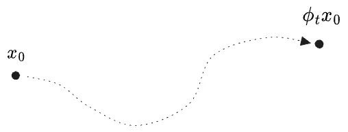
Let us denote the operation of “evolve in time by
For a given
The map of this motion under a function
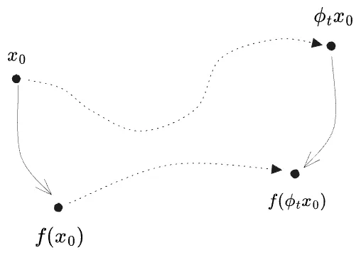
That is,
The “time-evolution” operator on functions, like
The time-evolved
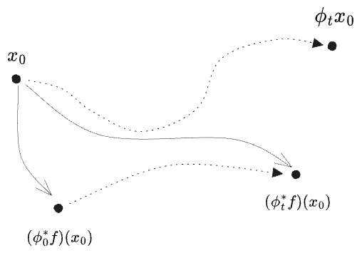
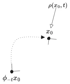
Whence the name “pullback”? We tend to think of
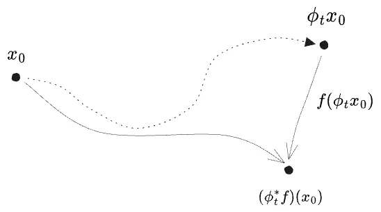
For a certain input point
or generally
where
In other words: if we regard
One effect of this definition is that
The “outermost” time-evolution composes to the right. This doesn’t really matter for the simple
Now for yet another view of time evolution. Frequently in physics we find ourselves wishing to think of a system being “in a state
where the “state” itself is a vector sum of “basis states” of specific
Here I’ve used a quantum-mechanics-inspired syntax to represent the states themselves, but such a description is generally used for representing any kind of “collection” of states—whether physically-real superpositions (as in quantum mechanics), epistemic ignorance (as in statistical mechanics), or hypothetical ensembles (as used in frequentist stat-mech). All the information is really contained in
For now we’ll limit ourselves to the single particle case
The delta-function case is easy, because the entire density is located at a single coordinate at all times. Let us see what it looks like first with a discretized time coordinate, where in an interval
Evidently the density
Visually:
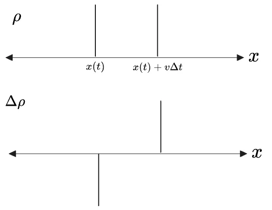
The answer looks like the negative derivative of a delta function,
For continuous-
The change in
What I’ve computed here is
Instead, by studying
In light of this we should go a step further and rewrite the above in terms of
we get
The last line is also the general formula for any
Compare with the rule we found for functions:
for which a formal solution
We will proceed another way. If we write an integral which measures the spatial average of a function
then if we were to study the time-evolution of this average, we should only time-evolve the argument to
Then writing
But now there appears a third option: keep
Here the
Apparently, if we want to assign the time-dependence to
In terms of our diagrams,
Our
is called the “pushforward”3 of
One last note. Pushforwards of densities turn out to compose in forward order,
like points
In all we have three “views” of time evolution:
- Trajectories
. - Functions
. - Densities
, which we think of as being associated with “states”
Note that these all describe the same evolution—we cannot really even say which view is primal! While the evolution of trajectories is the most natural pedagogical starting point, there is nothing in the physical world to truly distinguish this from, say, an opposite-in-time-variation of the function we use to measure or observe the state.
It turns out that “functions” and “densities” will be easier to talk about than “trajectories” themselves. Outside of the setting of
These representations are the natural material of physical theories. The “Heisenberg picture” of Quantum Mechanics is a description of time-evolving functions, and the Shrodinger picture of time-evolving states; approximately densities. (It is not a description of trajectories themselves, but as we saw trajectories and states both evolve in the “forward” direction, and a state is a trajectory in a larger space.)
Time-Ordered Exponentials
Now for one final feature frequently seen in physical theories which, it turns out, arises in the analysis of generic first-order systems.
Return again to our original ODE in one dimension, but now with a time-dependent velocity field:
If we discretize time into
The true trajectory should look like a
We could express the discretized solution on functions
(Note the pullbacks
Which will be easiest to calculate? If we try to integrate
and then we could imagine writing
For a general expression, it’s simplest to work on the pullback
where in the last line I’ve used
Forgetting about the particular
It will be useful to give the combination
Note that
With this, the operator equation is
The
We can now try to solve this “operator ODE” to find an explicit form of
which worked in the case of
but this is suspicious with
What we get has terms of
We can make progress by recursively applying the fundamental theorem of calculus for the operator
This is a fairly tidy infinite-sum-of-nested-integrals, at least. Note that the integration variables obey
Observe also that each
Therefore if we simultaneously…
- modify each integral to the full domain range
, multiplying the overall integration volume by - replace the products-of-
operators with a “reverse time-ordered product” , such that the operator argument always appear in the order of increasing time, even when the time parameters range into the region we just added to the integral, - and divide by
to undo the overcounting introduced by the first two steps…
… we should get an equivalent expression which even better resembles a true exponential series, and is therefore called the “(reverse) time-ordered exponential”:
This, finally, is a general solution to time evolution, albeit an unwieldy one. The reverse time-ordering operator
The most interesting thing about this is that the
I chose to work out the time-evolution of a function because the equivalent derivation for
If we imagine taking the spatial average of a function
then it should be possible to rewrite this integral with a different time-evolution operator applied to
What is the adjoint of
We move
Therefore
Note this is basically the r.h.s. of the equation for
We can immediately write down the general form of the pushforward time-evolution operator on densities:
Here we use a normal time-ordering because
But the operator
The first term is exactly the negative of
(Here I’ve switch the sign of the upper limit, reversed the time-ordering, and added a negative sign all at once. Effectively this is taking
The second term is simply a multiplication by
Therefore there must be some way to factor the time-ordered exponential of the first term of
What must be the expression for
Effectively this just adds up all the divergence in
In all:
where the first term is
Was this worth it?
Well, here’s the whole point: the standard description of classical mechanics is as the “time evolution of a density function”, though it is simplified somewhat by the Jacobian being
And even quantum mechanics can be described in this way, if you treat the real and imaginary parts of the wave function as distinct variables
My hope in the next post is to describe these three theories—classical mechanics, quantum mechanics in
-
I find this naming counterintuitive, as I am for some reason prejudiced to trying to read
as “pulling back”, or perhaps as “pulling back” (to , I suppose), rather than pulling its argument, the function , back. ↩ -
It’s curious that multiplication-by-
acts like a “width” here. Multiplication feels like the wrong sense for this. In the discrete case, would be approximately —it moves the mass between two bins a distance apart. But nothing would be multiplied… ↩ -
Only at this point did I realize that this “pushforward” is different from the first thing by that name one encounters in differential geometry, the linearization
which carries tangent vectors or vector fields along a general map . These are related, but this in fact is the same “pushforward of a measure” that one encounters in probability theory, e.g. when “pushing forward” a probability measure from a sample space to the real line by a random variable . ↩ -
I am certain I have seen a combinatorial-species-like derivation where the series of sequences of
terms in the exponential is combinatorially equivalent to another series generated by the exponentiation of the combination , an “interaction picture”-like expression. But with all the integrals this gets very hairy, and the final result turns out to be simple anyway. ↩