Entropy of Joint Distributions
Table of Contents
1. Independence
In the previous post we saw that the entropy of a product distribution
The above expression does not generalize to arbitrary joint distributions like
The entropy of a joint distribution is for for reason given its own name, the Joint Entropy, and has its own notation in terms of random variables:1
If
This is a bit reminiscent of the variance, which has a similar property for sums of independent distributions:
For non-independent distributions the variance behaves like a vector squared-norm
What happens to the entropy for non-independent distributions?
We can start by rewriting the joint distribution in terms of a conditional, which is exact:
where in the last line we’ve used the conventional notation
From this we can observe:
- if
is independent of , then and the conditional entropy reduces to the entropy of alone:
which recovers the additive property
- on the other hand, if
is completely determined by , then takes a single value on each level set of . The marginal distribution is an indicator , which makes the entropy of every marginal distribution, and the conditional entropy, zero:
We see that, for completely-dependent
The joint entropy in always less than the independent case:
A number of the qualitative properties of entropy follow from these observations.
- Correlations and “internal structure” always reduces entropy (while they tend to increase variances). In the extreme case of total dependence, they reduce a joint distribution of two variables into a single-variable distribution.
- Expanding a sample space along a new dimension can only increase the entropy:
. - Conditioning, such as with new “information” or “evidence”, can only reduce an entropy:
- Entropy is “concave” over probability distributions:
(this is an instance of Jensen’s Inequality) - Equivalently: whatever the entropy w.r.t. a specific distribution, uncertainty in the distribution itself will increases the entropy.
The last property is illustrated by the case of a biased coin distributed
which follows from the concavity formula with
We may conclude this discussion with one more concept, the mutual information, which is nothing but the difference between the joint entropy
If we characterize
2. Entropy as Measure?
A “Venn diagram” is useful to organize the preceding ideas:
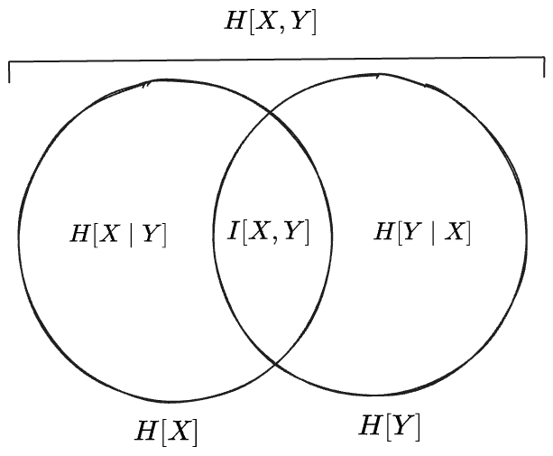
But, note, that while this diagram suggests an interpretation of entropy as the “measure” or “size” of some set—since Venn diagrams depict schematically the relationships between sets subsets—there exists no set of which these various entropy expressoins are measures. Instead we made the “Venn diagram” work by defining the mutual information
Interestingly, though, Taylor series of the entropy expression
and the first term in this series is the measure of something. If we consider the distribution
This expression admits an interpretation as the fraction of all pairs
The full sum
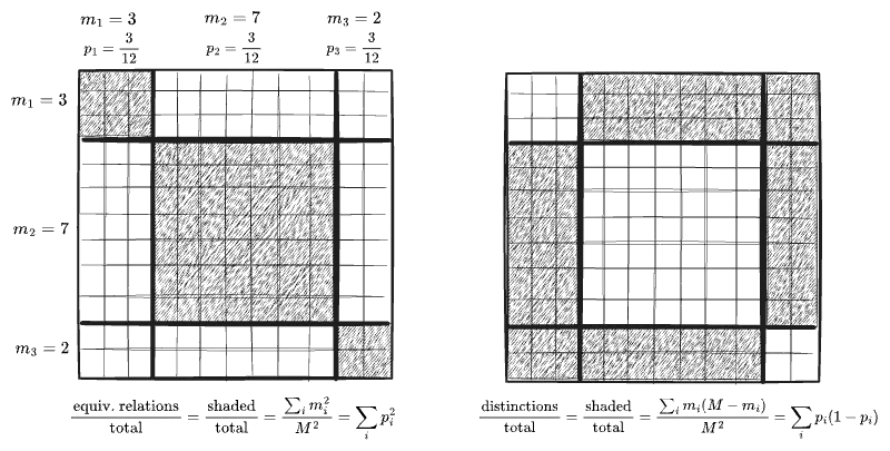
Therefore the first term in this “series” expansion of
The expression
-
Elsewhere we’ll see the notation
for the “cross entropy” of two distributions, with probabilities for arguments and an entirely different meaning. I prefer to use only probabilities like as arguments to entropy rather than random variables to avoid this kind of confusion. ↩ -
The intuition here that independent distributions add “at right angles”, each contributing only its own randomness, while correlated distributions “constructively interfere”. See my post on variances for more. ↩
-
An equivalent form is
, which in other contexts is known as the Gini impurity or Simpson diversity index. ↩
Comments
(via Bluesky)