Here we’ll pick up the thread from the previous post and try to figure out exactly what we’re talking about when we write an expression like

Table of Contents

• Flows
• Pullbacks
• Pushforwards
• In Summary

Flows

We first tried to describe the time-evolution of a single function with initial condition , the way one learns to do in a first differential equations course. The result was a direct integration

This worked for , but when we tried to take on we found that the derivation lead us to a different view of time-evolution as an operator , most easily understood as acting on functions of :

(I’m writing as a dot product to indicate it should work in any number of dimensions.)

If we think about it, the first case, whose solution simply added something to , clearly cannot be very general—in most spaces where one might want to describe the time-evolution of points, one cannot “add” points at all. We need some kind of “lens” onto the space—some way of viewing it without speaking directly of points.

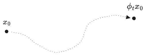
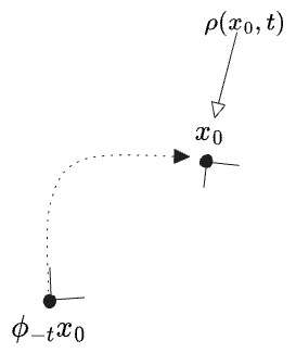
One such lens is the mapping induced by time-evolution itself. Let us denote the operation of “flow an initial point in time by ”, with a suitable manifold, by the “flow map”

For a given , maps initial points to time-evolved points:

obviously composes additively, since “times” are just real numbers:

The inverse of simply has the negative of the time:

In terms of , our original differential equation becomes

This must hold for any initial point , so we the two maps and are equal pointwise. We can therefore write a differential equation for itself,

We started with an ODE on points; now we have an diff. eq. on . Again this looks like something we could exponentiate:

but it’s not clear at this point what this means. If we were to expand the exponential in a series, even infinitesimally:

we would once again need a notion of “addition” on points. And terms of higher order would have factors , , meaning what? Repeated multiplication? Function composition?¹

To make progress we need to work with some we can do addition and multiplication with…

Pullbacks

… like functions.

The time derivative of a function (or any vector space we can add in) gives another ODE:

In the previous post we worked out the operator which implements time evolution on functions:

We could also have derived this by repeatedly substituting with the fundamental theorem of calculus,

This is a true power series, with addition in the output space of and multiplication as composition of differential operators.

If we express the ODE for in terms of , we have

We can omit the initial point to get at an equation which should hold pointwise:

This almost looks like somethingwe can solve directly for the “time-evolution operator on functions” we just wrote down. We need to drop the specific function , reminiscent of how we droppped the initial point from earlier.

Let us briefly study the object . The image of the map under a function is some trajectory in :

That is,

The “time-evolution” operator on functions is an operator which takes a function to the new function . This is a mapping of functions to functions, called the “pullback” of , denoted :

The time-evolved will be the function taking an initial point to its endpoint after :

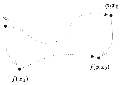
Whence the name “pullback”? We tend to think of as “pushing” or “flowing” the point according to an evolution law, with a sense of evolving “forward” in time. Then compare and :

For a certain input point , whose output under is , the input point which would produce the same output under is simply , the point which precedes under time evolution by . That is, for and both nicely invertible,

or generally

where and may be sets rather than single points.

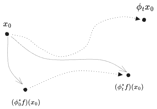
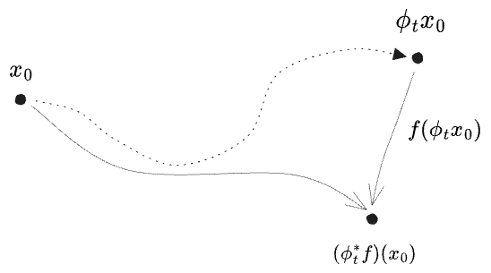
In other words: if we regard as a simple directed arrow between points in and , then moves the initial tip of backwards along lines of time-evolution in —the end of the arrow is “pulled back” in time.²

One note: composes times oppositely to itself:

The pullback at the later time is on the right.

---

Returning to the equation

we now see that both sides may be written as a pullback,

Now the function itself is the rightmost term on each side, and we can omit it to arrive at a differential equation for the pullback itself,

We already know the solution for velocities ; it is just the exponential which implements the appropriate series expansion on functions of :

Pushforwards

Now for yet another view of time evolution. Frequently in physics we find ourselves wishing to think of a system being “in a state” which is some vector some of of all possible states , where the entire state evolves with time, rather than as being described by a single point moving with time. In this view a one-dimensional trajectory might be written , which represents a moving delta function

This description has the advantage of readily generalizing to non--function states with arbitrary “densities” ,

Here I’ve used a quantum-mechanics-inspired syntax to represent the states themselves, but such a description is generally used for representing any kind of “collection” of states—whether physically-real superpositions (as in quantum mechanics), epistemic ignorance (as in statistical mechanics), or hypothetical ensembles (as used in frequentist stat-mech). All the information is really contained in , and we could skip writing the state vectors to give it more of a stat-mech feel:

For now we’ll limit ourselves to the single particle case .

Given that the trajectory is known (it is defined by our original ODE ), how should we represent the evolution of , and specifically of the density ?

The delta-function case is easy, because the entire density is located at a single coordinate at all times. Let us see consider first the case where the time is discretized, such that in an interval the particle moves as

Evidently the density must change in such a way that it removes all of the density from and adds it all to . The exact change in would be

Visually:

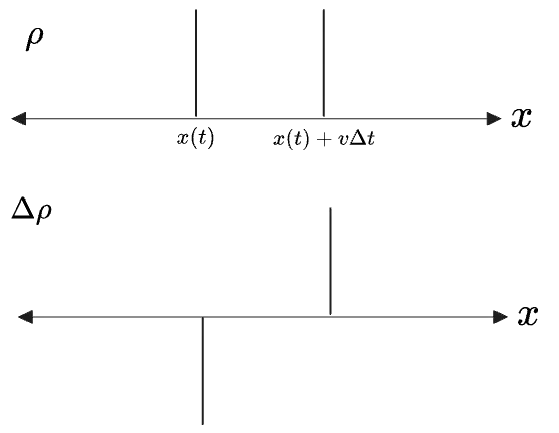
The answer looks like the negative derivative of an indicator function, , with “width” . This is easy enough to express in a discrete setting—but continuously?

For continuous- case, still for a delta-function density:

The change in is exactly a delta-derivative multiplied by a “width” .³

What I’ve computed here is . This is because, contrary to the case of , we do not want to follow the flow of the density . An expression like treats as a “pointer” moving through the space , with measuring the value of at the point pointed-to, and the change in this value. If we did the same for the density we would be treating it as if the density were fixed in space as a function , and the only change with time would come from the explicit time variation of the underlying point .

By studying instead, we are fixing a point and gauging how changes with time due to the flow of under .

In light of this we should go a step further and rewrite the above in terms of rather than for a truly “local” evolution law for . Applying the -function identity

we get

The last line is also the general formula for any , though we’ve derived it only for the -function case.

Can we now write the solution to as an exponential?

Compare with the rule we found for functions:

for which an exponential solution could be written. The r.h.s. operator of the equation,

suggests an exponential

But this is a more complicated, as the two terms cannot be freely re-ordered.

The term, on its own, would exponentiate as ; evidently it translates backwards by . But the other term makes a mess of things.

---

We will proceed another way. If we write an integral which measures the spatial average of a function ,

then if we were to study the time-evolution of this average, we should only time-evolve the argument to . The part simply represents a fixed integral over the entire space, and should not evolve:

Then writing , we can see the earlier vs. distinction as associating the time-evolution operator either to the right or left:

But now there appears a third option: keep fixed but transform the coordinate of the entire integral backwards:

Here the term is the Jacobian of the time evolution map .

Apparently, if we want to assign the time-dependence to , what we need is:

In terms of our diagrams, simply “watches” a spot of the space as flows under it. The density at at is the density which was at at time . The following diagram represents this informally (with the little reference frame evoking the time-evolving volume element which produces the Jacobian term):

Our expression,

is called the “pushforward”⁴ of by , denoted :

Pushforwards of densities compose in forward order,

like points themselves (and unlike functions/pullbacks). This looks wrong at a glance, because the time-evolution operators are applied to the argument of in reverse order. But to find the density which flows into the point at time we should find the point to which application of gives , and this is exactly :

---

Let us now write a differential equation for the evolution of the pushforward itself.

We should begin with the evolution of a density,

Rewrite with a pushforward:

Omit the initial point for an equation which should hold pointwise:

Replacing and for a coordinate-free expression:

And now omit the density for an equation which should hold for all densities:

This is a linear operator on pushforwards , and should have a “solution”. If we write the r.h.s. as a generic linear operator , defined by

the previous cases suggest the solution will simply be

The difficulty now is that has two terms:

The second term looks exactly like diff. eq. for the pullback, , for which the solution was , except for the minus sign. On its own it would implement the factor in

which, at a time , looks at the density arriving from the earlier point .

The other term, which involves the divergence of the velocity , must produce the second Jacobian factor. It almost looks as if we could split the two terms of the integral apart. But we can’t:

or in any other order, for the usual reason that these two operators do not commute with one another. The Jacobian factor is not simply the divergence at the initial point—which makes sense; it should incorporate the divergences along the entire path.

Instead, a trick. Our differential equation for reads

Consider instead the “comoving density”

which gives, for a coordinate and time , the density which is “actually” at the coordinate .

The time derivative of is

Only the divergence term survives. We know the implements , so we can pull it into the other terms, re-introducing an explicit -dependence for and identifying again:

We cannot literally exponentiate this, , because depends on the current time. But the r.h.s. is a pure multiplication, so we can divide across and integrate:

We get, not a pure exponential, but an exponential-integral, which picks up all velocity divergences along the flow. We can then write itself:

In the third line I combined and then replaced inside the integral. In the last line I replaced , since at .

This is our pushforward operator:

or simply

By the integration-by-parts argument from before we know should have the form , meaning that we can identify the exponential-integral with the Jacobian:

Evidently the Jacobian is the accumulation of divergences in the velocity field which would have been encountered along the trajectory in the time . The negative sign in the exponential represents the fact that a divergence in the past should shrink the density at the current time, as a divergence represents a spreadin-out of trajectories.

In Summary

We began with the elementary view of time evolution as a “trajectory” . Now we have three more ways of looking at it. In a table:

Note that these all describe the same evolution—we cannot really say any one view is primal! While the evolution of trajectories is the most natural pedagogical starting point, there is nothing in the physical world to truly distinguish this from, say, an opposite-in-time-variation of the function we use to measure or observe the state.

We have still not considered a time-dependent velocity . That will next, and will complicate things somewhat.

---

Footnotes

1. The best choice might be to take as a definition of the exponential of the flow map resulting from a vector field . My understanding is that this is done, but the notation employed is , a different but related object, which is not taken to have a series expansion. Only when applied to functions (as the pullback , discussed further on) does it becomes (if we understand to act on functions as a directional derivative) or (if we want to be explicit), with a series expansion. ↩

2. I find this naming counterintuitive, as I am for some reason prejudiced to trying to read as “pulling back”, or perhaps as “pulling back” (to , I suppose), rather than pulling its argument, the function , back. ↩

3. It’s curious that multiplication-by- acts like a “width” here. Multiplication feels like the wrong sense for this. In the discrete case, would be approximately —it moves the mass between two bins a distance apart. But nothing would be multiplied… ↩

4. Only at this point did I realize that this “pushforward” is different from the first thing by that name one encounters in differential geometry, the linearization which carries tangent vectors or vector fields along a general map . These are related, but the present pushforward is really the same “pushforward of measure” one encounters in probability theory, e.g. a random variable pushing a probability measure forward from a sample space to the real line. ↩